# Week 6 - Graph algorithms - strongly connected components
Last edited: 2023-11-11
# DFS - not the sofa seller!
Recall the definition of Depth-first search (DFS) in the note. We used it there to find the connected components of a graph.
DFS to find connected components in an undirected graph
# Find paths in undirected graph via DFS
First for undirected graphs we just keep track of the previous vertex and find a spanning sub -forest for the graph . We can use this to find paths between vertices by going back to the root vertices of the trees .
DFS(G)
  input: G = (V,E) in adjacency list representation
  output: Vertices labelled by connected components
    connected_component = 0
    for all v in V, set visited(v) = False, previous(v) = Null
    for all v in V
      if not visited(v) then
        connected_component++
        explore(v)
    return previous
Explore(z)
  input: vertex z
    connected_component_number(z) = connected_component
    visited(z) = True
    for all (z, w) in E
      if not visited(w)
        previous(w) = z
        Explore(w)
# Find paths in undirected graph via DFS
To do this we are going to use a DFS algorithm like above but we are going to track pre/postorder numbers.
DFS(G)
  input: G = (V,E) in adjacency list representation
  output: Vertices labelled by connected components
    clock = 1
    for all v in V, set visited(v) = False
    for all v in V
      if not visited(v) then
        explore(v)
  return post (defined in Explore)
Explore(z)
  input: vertex z
    pre(z) = clock, clock ++
    visited(z) = True
    for all (z, w) in E
      if not visited(w)
        Explore(w)
	post(z) = clock, clock++
# Example
Suppose we have the following graph and let $B$ be the root node. Suppose we explore edges alphabetically and lets run the algorithm above on it.
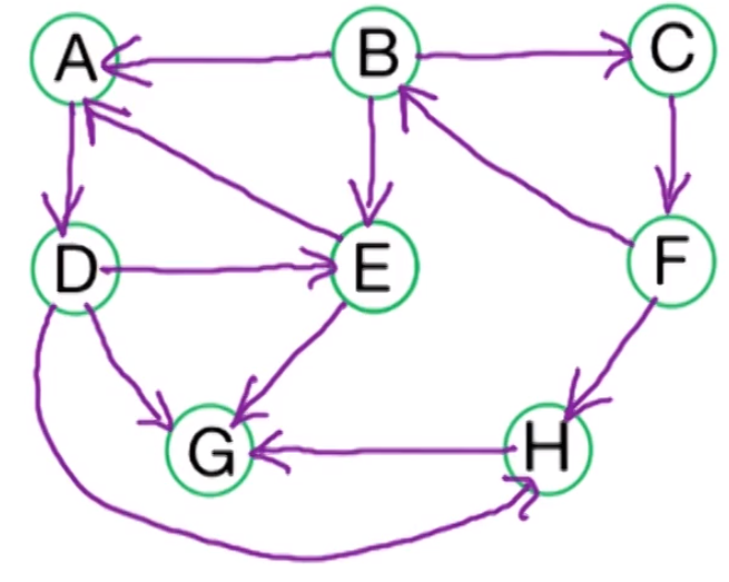
As we are using DFS we explore far first and then slowly come back. Which gives us the following DFS tree with the pre/post numbers.
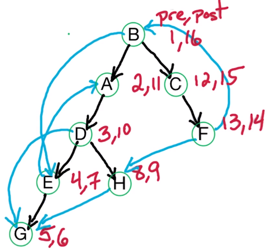
| Letter | Pre | Post |
|---|---|---|
| A | 2 | 11 |
| B | 1 | 16 |
| C | 12 | 15 |
| D | 3 | 10 |
| E | 4 | 7 |
| F | 13 | 15 |
| G | 5 | 6 |
| H | 8 | 9 |
Lets try and classify the edges $(z,w)$ in this graph
- Tree edges
- Back edges
- Edges going from a node further out from the root (in the black edges) to a node closer to it but still in the same branch.
- Examples $E \rightarrow A$, $F \rightarrow B$
- $post(z) < post(w)$
- Forward edges
- Edges that go further down the tree.
- Examples: $B \rightarrow E$, $D \rightarrow G$
- $post(z) > post(w)$
- Cross edges
- Edges that go from one branch to another.
- Examples: $F \rightarrow H$, $H \rightarrow G$
- $post(z) > post(w)$
Note here there the only type of edges to have $post(z) < post(w)$ are back edges.
Cycles in a graph via the DFS tree
# Topological sorting
Suppose we have a DAG $D$ from the lemma above we can run a DFS algorithm starting at the root of $D$ and the post ordering will provide a topological sorting of the vertices of $D$.
# Vertices in a DAG
We can classify special vertices in a DAG
- Source vertices: These have no incoming edges
- Sink vertices: no outgoing edges
Given a linear ordering we know the minimal vertex is a source and the maximal vertex is a sink. This gives us another algorithm to find a topologically sorting :
- Find a sink vertex, label it and then delete it.
- Repeat (1) until the graph is empty
# Strongly connected components
Recall the definitions
Then we can define the strongly connected component graph
strongly connected component graph
Which we can show is a DAG .
The strongly connected component graph is a DAG
# Strongly connected component algorithm
The idea of the algorithm is the following:
- Find a sink strongly connected component ,
- Remove it,
- Repeat!
We use sinks as if we start a DFS algorithm in a sink strongly connected component we only discover vertices in that strongly connected component .
This is not true for source strongly connected components , here we discover everything.
# Finding a vertex in a sink SCC
We have the following two statements in a DAG :
- The vertex with the lowest postorder number is a sink.
- Then vertex with the highest postorder number is a source.
We would hope for the analogous statements in a general directed graph :
- The vertex with the lowest post order number is in a sink strongly connected component
- The vertex with the highest post order number is in a source strongly connected component
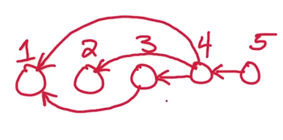
The first statement is false consider the following counter example.

If we run a DFS algorithm starting at $A$ using an alphabetical ordering on the vertices then $B$ has the lowest post order number but is in the source strongly connected component .
A vertex with the highest post order number lies in a source SCC
Suppose we a directed graph $G$ define the reverse directed graph $G^R$. Now observe
The strongly connected components are the same in a directed graph and its reverse
Moverover we have.
Taking the reverse respects going to the strongly connected component graph
Therefore if we can find a source vertex in $S_{G^R}$ then we have found a sink vertex in $S_G$. This is exactly what our algorithm will depend on.
# Algorithm for finding the strongly connected components
SCC(G):
	Input: directed graph G = (V,E) in adjacency list
	Output: labeling of V by strongly connected component
		1. Construct G^R
		2. Run DFS on G^R
		3. Order V by decreasing post order number.
		4. Run directed DFS on G using the vertex ordering from before and
		   label the connected components we reach.
In addition to labelling the connected components the order we have labelled them is in reverse topological ordering. This is because we always start at the next sink vertex after we have labelled a component.
This takes $O(\vert V \vert + \vert E \vert)$ as we do two runs of a DFS algorithm.
# Example
Suppose we want to find the strongly connected components of the graph $G$ below.
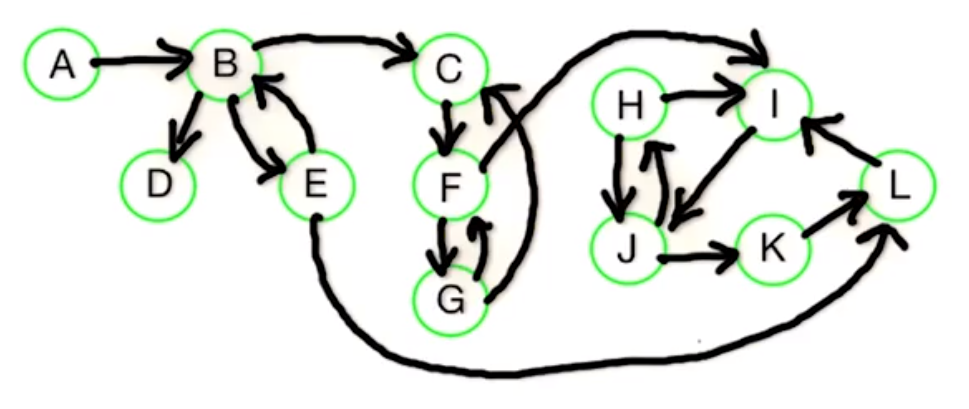
First we look at $G^R$ and run the DFS to find path in an undirected graph algorithm.
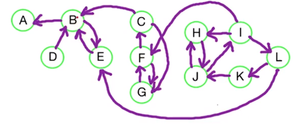
This gives us $post : V \rightarrow \mathbb{N}$ - in this example we started at $C$ and did a fairly random vertex ordering.
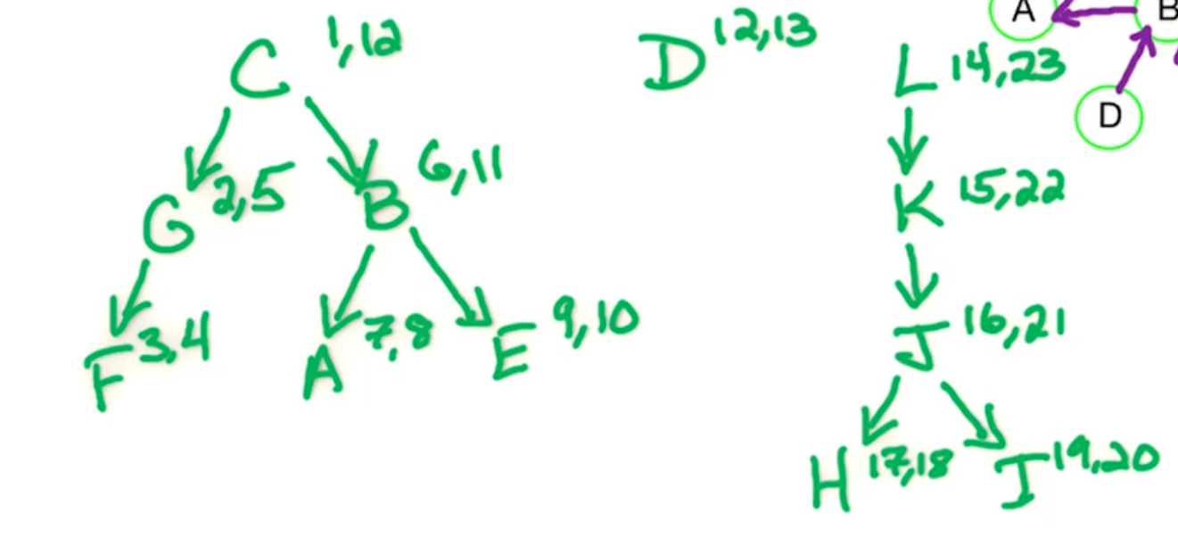
| Letter | Pre | Post |
|---|---|---|
| A | 7 | 8 |
| B | 6 | 11 |
| C | 1 | 12 |
| D | 12 | 13 |
| E | 9 | 10 |
| F | 3 | 4 |
| G | 2 | 5 |
| H | 17 | 18 |
| I | 19 | 20 |
| J | 16 | 21 |
| K | 15 | 22 |
| L | 14 | 23 |
Then we order the vertices by reverse post order.
| Letter | L | K | J | I | H | D | C | B | E | A | G | F |
|---|---|---|---|---|---|---|---|---|---|---|---|---|
| Post | 23 | 22 | 21 | 20 | 18 | 13 | 12 | 11 | 10 | 8 | 5 | 4 |
Now run a connected components DFS using the vertex ordering above.
| Letter | L | K | J | I | H | D | C | B | E | A | G | F |
|---|---|---|---|---|---|---|---|---|---|---|---|---|
| Post | 23 | 22 | 21 | 20 | 18 | 13 | 12 | 11 | 10 | 8 | 5 | 4 |
| CC | 1 | 1 | 1 | 1 | 1 | 2 | 3 | 4 | 4 | 5 | 3 | 3 |
Notice also that the strongly connected component graph is the following.
Giving that our ordering is exactly a reverse topological sorting .