# Week 8 - Distributed memory model
Last edited: 2026-05-27
In this lecture, we are going to look at computations that involve so much memory that they cannot fit on a single computer and instead need to use a distributed set of computers or would take years to compute alone. In the distributed setting each computer has its own memory and can only communicate with others via message passing.
# Distributed memory model
In our model we have a set of ‘machines’ which involve:
A single processor.
Private memory.
The private memory cannot be read by any other machine and will need to be sent to another machine if it is needed. These machines are connected in a network - which can have an arbitrary structure. This model follows some rules:
The network is fully connected - and any computer can talk to any other computer.
All links in the network are Bidirectional.
Nodes can concurrently send and receive at most 1 message at a time.
The time to send a message of $n$ words in an uncongested network is $T_{msg}(n) = \alpha + \beta n$. Here we call $\alpha$ the latency and $\beta$ the inverse bandwidth.
k-way congestion reduces bandwidth to $T_{msg}(n) = \alpha + \beta n k$. Note, this is only if the messages are going in the ‘same’ direction - messages going in opposite directions don’t compete by rule 3.
Note how rule 4-5 are ‘path’ independent up to congestion. This is counterintuitive because in physical networks, the path length typically matters.
# Message cost justification
Suppose we have a linear set of machines of length $P$ and we need to send a word of length $n$ from the first to the last machine. Suppose there is a fixed cost of getting ready to send a message $a$ and a time $t$ for the message to pass between two machines. Lastly lets say we can only send 1 word at a time and machines can send/receive 1 word at a time. Then the first machine will send off each word 1 at a time and the rest of the machines will act as a relay. The first message will take $a + (P-1)t$ time to get there, with the kth message taking $a + (P-1)t + kt$ time.
Roughly we group $(a + (P-1)t)$ as $\alpha$ and $t$ as $\beta$. However, you might think $\alpha$ isn’t really a constant then - as it depends on $P$. Here we assume that $a >> (P-1)t$ as $t$ should be small in comparison to $a$. Therefore by some fuzzy logic we say this makes it a constant.
# Relative costs
In this model we have two parameters $\alpha$ latency measured in time per message, and $\beta$ inverse bandwidth measured in time per word. In the computational model there is another ratio that is important, $\tau$ which is compute, i.e. time per operation.
Here we have $\tau << \beta << \alpha$, in terms of orders we normally see $\tau = 10^{-12}$, $\beta = 10^{-9}$ and $\alpha = 10^{-6}$. From this we get two important observations:
Compute is much faster than message passing.
Also sending fewer larger messages is cheaper than many small messages.
# Primitives
In this model there are core fundamental operations that lots of higher level algorithms use. These are interesting to study to understand payoffs within this model and how to think about message passing.
To write pseudocode for these we use the single-program, multiple-data (SPMD) model. Here we have 1 piece of code that runs on multiple processes. To differentiate the processes we use:
P: The total number of processes.RANK: The process id, normally 0 toP-1.
Here to use message passing we have the asynchronous operations:
sendAsync(buf[1:n], dest): This marks the data inbufto send to node with rankdest, this returns a handle we can use to check the status of this.recvAsync(buf[1:n], source): This marks the data inbufto receive data from node with ranksource, this returns a handle we can use to check the status of this.wait(handle): This waits for the handle to be ready or you can provide a null handle which waits for all handles to be ready. This just tells us that thebufis now safe to use again.
Just because we have called sendAsync or recvAsync, does not mean the data has been sent or received. You must wait for that to happen before interacting with buf again.
The implementation of sendAsync or recvAsync is up to the underlying software.
Therefore, we cannot make any assumptions about how it is implemented, which means sendAsync may block until it has been received, causing a deadlock if not thought through carefully.
Similarly, we cannot assume the receiver has received the message just because sendAsync has returned, as it may have simply copied the data to the NIC.
# All-to-one Reduce
Suppose we have $P$ machines all with an array of length $n$. We want to reduce these arrays into a single one. To do this we are going to implement a ’tree’ reduction where we pair machines together. Then the result will end up in one of the pair leaving half as many machines for the next round.
To assist with the pairing process we are going to consider the RANK of the machine in binary.
Starting with the least significant bit we pair machines that agree on the other bits.
Then the machine with a 0 in that bit becomes the receiver for the reduction and the machine with 1 in that bit sends its data.
In subsequent rounds we shift the bit we look at - then only machines with 0’s before this bit have data.
allToOneReduce(buf[1:n], root = 0):
  bitmask = 1
  while bitmask < P:
    PARTNER = RANK ^ bitmask       // XOR the bits
    isSender = RANK & bitmask      // logical AND the bits
    if isSender != 0:
      sendAsync(buf[1:n], PARTNER)
      wait(*)
      break                        // Senders no longer needed
    else if PARTNER < P:           // If your partner does not exist skip
      temp is array of length n
      recvAsync(temp[1:n], PARTNER)
      wait(*)
      buf = localReduce(buf,temp)
    bitmask = bitmask << 1         // Shift the bit
  if RANK == 0:
    return buf
This takes $O((\alpha + \beta n) \log P)$ time to complete, assuming all nodes are connected in a linear fashion with node $i$ connected to nodes $i-1$ and $i+1$.
# One-to-all Broadcast
A dual to reduce is broadcast, where we send data from one node to all other nodes.
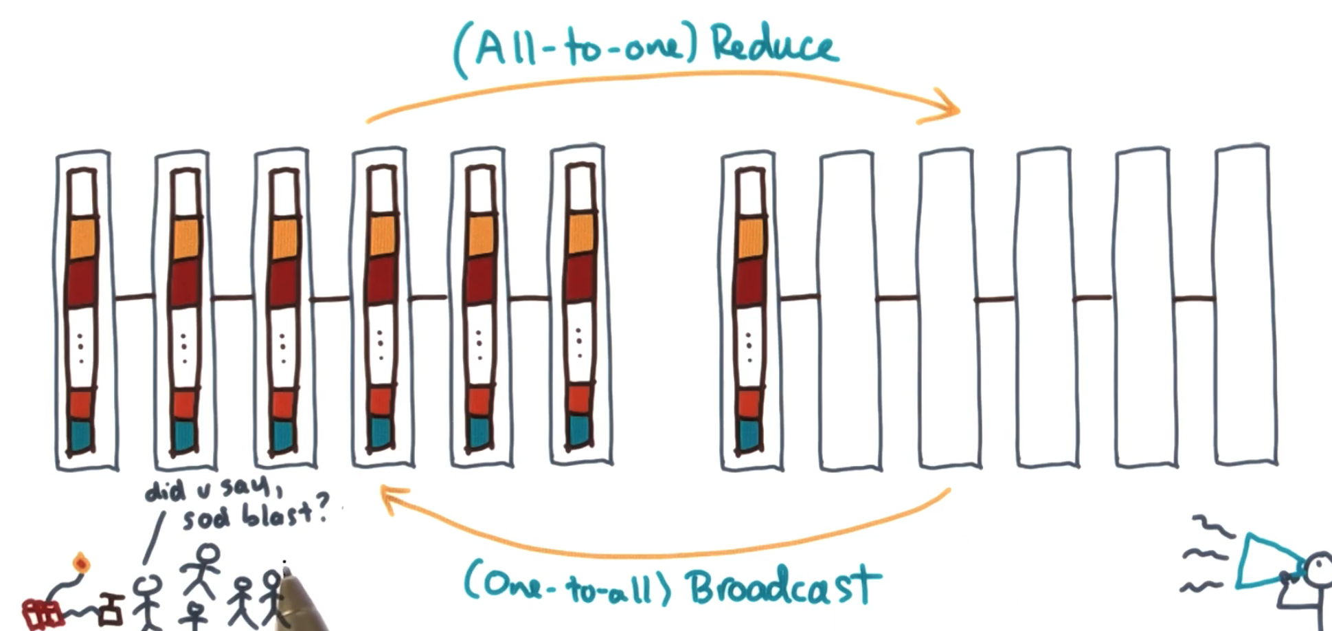
Note that they are not complete opposites, as you are not undoing the reduction to get the original slices back.
This can be implemented in a similar way to reduce, but we will come back to if this is the optimal way to do it.
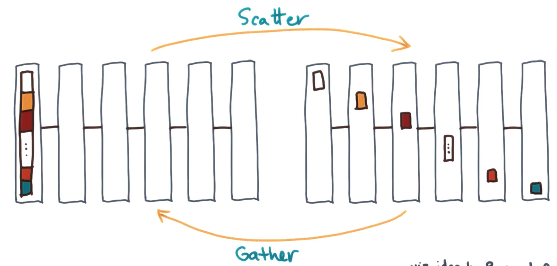
# Gather and Scatter
Gather and scatter are real opposites of one another. Gather gets data from every node and gathers it onto a single node. Scatter takes data from one node and separates it up to all the other nodes.
# All-gather and reduce-scatter
All gather is similar to the gather but the data ends up on all machines at the end. A reduce scatter is the combination of a reduce with a scatter. Initially there is data on all machines and a reduction operation is applied to it. Then that data ends up split up into chunks on all the machines involved.
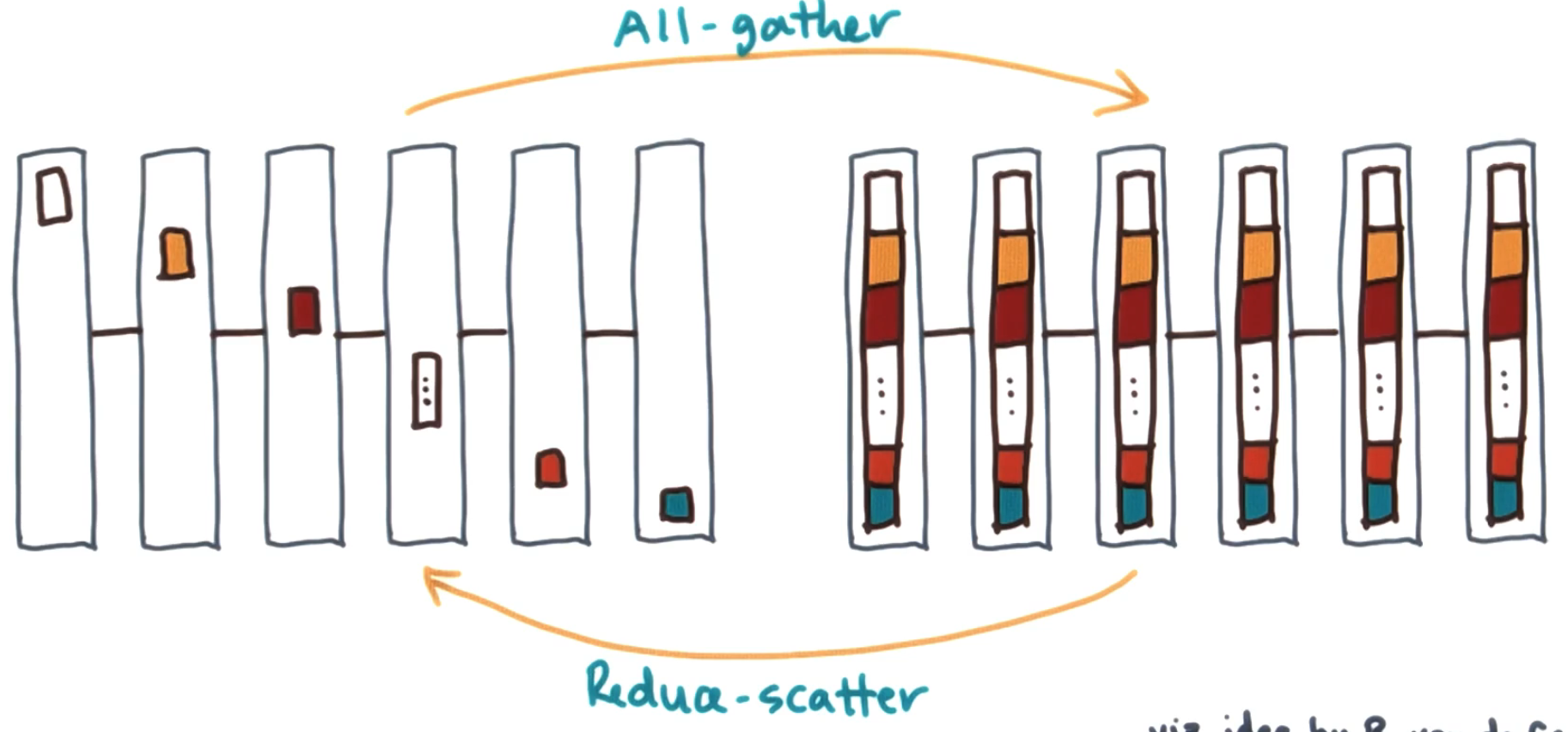
Whilst reduce scatter might feel counter intuitive - imagine working on massive data you need to do some complex operation on. Here you separate the data onto different machines to carry out that operation on, whilst reducing it.
# API
These primitives are called often, so we establish standard APIs for them.
allToOneReduce(buf[1:n], root): For each machine they have abufand they will reduce this data across all the machines toroot.oneToAllBroadcast(buf[1:n], root): For each machine they have abufand they will broadcast this data to all the machines from therootmachine.gather(In[1:m], Out[1:m][1:P], root): Each machine holds their slice inIn[1:m]and therootmachine stores the output inOut[1:m][1:P].scatter(In[1:m][1:P], Out[1:m], root): Therootmachine holds all the data inIn[1:P][1:m]and all other machines have their slice stored inOut[1:m].allGather(In[1:m], Out[1:m][1:P]): Each machine holds their slice inIn[1:m]and stores the output inOut[1:m][1:P].reduceScatter(In[1:m][1:P], Out[1:m]): Each machine holds their input data inIn[1:P][1:m]and has their output saved inOut[1:m].
For some operations we use $m$ instead of $n$, we do this assuming $n = mP$, so for analysis we can stick with $n$ as the size of the input/output.
There are 2d and 1d arrays in these operations and it will be convenient to go between them so we introduce an API to do this.
reshape(In[1:m][1:P], Out[1:n]): This reshapes the input array into the output array.reshape(In[1:n], Out[1:m][1:P]): This reshapes the input array into the output array.
This does not actually change the data in anyway but allows us to index it in a more intuitive manner.
# Efficiency
In the tree-based reduce we described earlier we took $O((\alpha + \beta n) \log P)$. Is this good or not?
Starting on the left hand side of $\alpha \log(P)$ the question becomes do we need $\log(P)$ rounds of messages? As all messages go from 1 machine to another and they are set up in linear lines the very best we can do is $\log(P)$ rounds as we need to merge $P$ bits of information. Each round we can at best merge pairs of information.
Next let us look at the right hand side of $\beta n \log(P)$ - this means we are sending $n$ words $\log(P)$ times. For an optimal lower bound consider what information needs to be sent $(P-1)n$ words (i.e. every process needs to send their $n$ words to the root). If each of the processes could send their data at the same time we would parallelise this and get the best time to be $\beta n (P-1)/(P-1) = \beta n$ time. Therefore we could say that our algorithm is ‘sending too much data’ by a factor of $\log(P)$.
This logic holds for all the processes we have above so the optimal time is always $\Theta(\alpha \log(P) + \beta n)$.
# Optimal Scatter/Gather
In the reduce case we saw that $\log(P)$ rounds of communication was optimal but we sent too much data. We want to use this insight to see if we can achieve a better Scatter/Gather - let us implement Scatter then Gather is the reverse of it.
The idea is similar to tree reduce - however we are going to do it in reverse and divide and conquer along powers of 2. First push half the data to the second half of the machines then iterate.
// For this assume P = 2^k
Scatter(In[1:m][1:P], Out[1:m], root = 0):
  mask = 2^(k-1)      // This looks like 100..0
  check = 2^{k-1}-1   // This looks like 011..1
  for i = 1 to k:
    if (check & RANK) == 0:
      partner = RANK ^ mask
      toRecv = mask & RANK
      chunkSize = 2^(k-i)  // This is the same value as mask but we used a new name to make it clearer.
      if toRecv == 0:
        sendAsync(reshape(In[1:m][RANK+chunkSize:RANK + 2*chunkSize]), partner)
        wait(*)
      else:
        temp = array of length m*chunkSize
        recvAsync(temp[1:m*chunkSize], partner)
        wait(*)
        reshape(temp[1:m*chunkSize], In[1:m][RANK:RANK+chunkSize])
    mask = mask >> 1    // Shift the mask down
    check = check >> 1  // Shift the check down
  Out = In[1:m][RANK]
This still takes $O(\log(P))$ rounds of communication. However, in each round we are only sending $n \cdot 2^{-i}$ words in each communication. Therefore, assuming no interference (due to the linear topology assumption), we get $T(n) = \sum_{i=1}^{k = \log P} \alpha + \beta n \cdot 2^{-i} = \log(P) \alpha + \beta n \frac{P-1}{P} = O(\log P \cdot \alpha + \beta n)$. This achieves the ideal bound on this type of primitive.
# Back to reduce
We saw earlier that reduce runs in $O((\alpha + \beta n) \log P)$ time. Is this actually bad?
There are two ways our algorithm could be inefficient: it could be operating on massive data or operating over many machines. If $\beta n \ll \alpha$ and $n$ is small, then $\alpha$ dominates our runtime, so the $\log(P)$ term on our $\beta$ does not matter as much, since just communicating is taking up all the effort.
# Bucketing (payoffs)
In some algorithms we can achieve better bandwidth efficiency by “bucketing” - breaking data into chunks and passing them incrementally rather than all at once. This trades off latency (more message rounds) for bandwidth (less total data movement).
Next let us look at allGather. There is a simple way to implement allGather: run gather followed by broadcast. From above, this would run in $O((\log P \cdot \alpha + \beta n) + \log P (\alpha + \beta n)) = O((\alpha + \beta n) \log P)$. This is optimal in the $\alpha$ term, i.e. the number of communication rounds, but not optimal in terms of the $\beta$ term. (Recall that this is acceptable if $n$ is small relative to $\alpha$ and $\beta$.)
Let us look at another way to implement allGather. The idea behind this algorithm is each process passes on the information they got in the last round (or start with in the first round).
allGather(In[1:m], Out[1:m][1:P]):
  Out[1:m][RANK] = In[1:m]
  for i = 0 to P-1:
    sendAsync(Out[1:m][RANK+i], RANK-1 % P)
    recvAsync(Out[1:m][RANK+i+1], RANK+1 % P)
    wait(*)
Here we have $P$ rounds, but each round we are only sending $m$ words.
That is, the runtime is $O(\alpha P + \beta n)$.
This is optimal in terms of the $\beta$ term but suboptimal in the $\alpha$ term.
This algorithm is better in the case where $n/P \ll \alpha / \beta$, i.e. the amount of data is our limiting factor.
We will call such algorithms bandwidth optimal.
A similar idea can be used for Broadcast by combining scatter and allGather.
broadcast(buf[1:n], root):
  chunked = 2d array of length m and P
  temp = 1d array of length m
  reshape(buf[1:n], chunked[1:m][1:P])
  scatter(chunked[1:m][1:P], temp[1:m], root)
  allGather(temp[1:m], chunked[1:m][1:P])  // Use the bucketed allGather version
  reshape(chunked[1:m][1:P], buf[1:n])
Since scatter is optimal and allGather is bucketed, this gives us a bandwidth optimal broadcast as well.
# Summary
This model is somewhat complex, and you will change algorithms depending on what the bottleneck of your algorithm is: the size of the data or the number of machines.