In this lecture we will look at speeding up Breadth-first search . In this lecture we will use BFS to find the distance of each vertex away from a root. The code for this algorithm might look like below:

BFS(G = (V,E), root):
  D : V -> Int
  D[v] = 0 if v = root else infinity
  F = { root }
  while F is not empty:
    v = F.pop()
    for all edges (v,w) in E:
      if D[w] = infinity:
        D[w] = D[v] + 1
        F = F union {w}
  return D

This has $W(G) = O(\vert V \vert + \vert E \vert)$ but is not very parallel with $D(G) = O(\vert V \vert)$. This algorithm is blocked from being parallelised by the set $F$ and function $D$ as it is edited on each pass through.

# Level parallel BFS

The output of this algorithm is a function $D: V \rightarrow \mathbb{N} \cup \{\infty\}$ that naturally partitions the graph into levels from the perspective of the root. Whilst processing nodes in each level the operations we do look the same. We identify nodes for the next level and give them that value. This will enable us to parallelise at these levels - as it does not matter if we process each one at the same time as they will not interfere with each other. This is summarised in the code below:

ParallelBFS(G = (V,E), root):
  D[v] = 0 if v = root else infinity
  level = 0
  F_0 = Bag{ root }
  while F_level is not empty:
    F_{level + 1} = { }
    ProcessLevel(G, F_level, F_{level + 1}, D)
    level = level + 1
  return D

ProcessLevel(G, F, F_next, D):
  if | F | > C then:
    (A, B) = bagSplit(F)
    spawn ProcessLevel(G, A, F_next, D)
    ProcessLevel(G, B, F_next, D)
    sync
  else:
    for v in F:
      par-for all edges (v,w) in G:
        if D[w] = infinity:
          D[w] = D[v] + 1
          bagInsert(F_next, w)

However, you may see we are ‘slightly’ cheating here as within the par-for’s we are updating D and F_next. All changes to D are to the same value - so a race condition here is not an issue. For changes to F_next - we will define a new data structure called a ‘bag’ where unions and splits are fast and atomic.

# Bags

A bag is an unordered set, that allows repetition. On this unordered set we will define the following fast operations:

• Traversal of the elements in a bag.

• Splitting a bag into two bags.

• A logically associative (A union B ~= B union A) union of two bags.

To implement this we will look at another sub-object.

# Pennant

A Pennant is a tree with $2^k$ nodes of the following form. It has a unary root with a single child. The child of the root is a complete binary tree of depth $k-1$.

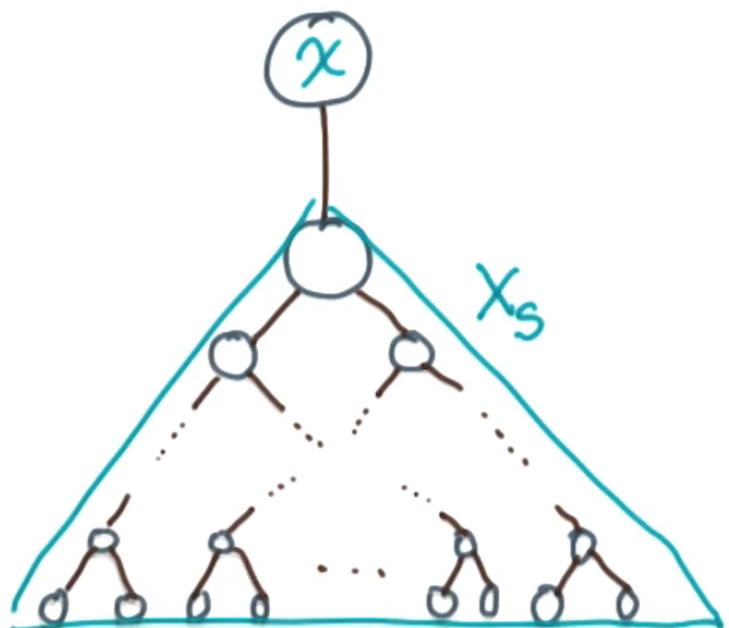
We can combine two pennants of size $2^k$ by:

1. Choosing one root as the new parent root
2. Making the other pennant’s root its child
3. Redistributing their complete binary subtrees to form a complete binary tree at the child root

If the two original pennants had size $2^k$ the new pennant has size $2^{k+1}$.

We can do the same operation but in reverse to make a pennant split. Here we take a pennant of size $2^k$ and split it into two pennants of size $2^{k-1}$. The roots are the original root and the root of the complete binary subtree below it. Where their subtrees are the two branches of the original complete binary subtree.

# Spines

To use pennants to make a bag we will connect multiple of them together into a spine. Functionally a spine is an array of pointers $(p_i)_{i}$ where $p_i$ is either null or points to a pennant of size $2^i$. Think of a spine as a binary number - when a pointer is non null in position $i$ then you have $2^i$ elements. Meaning that the number of elements in the spine in base 2 is represented by a 1 if the pointer is non null and 0 otherwise.

# Spine unions

Given two spines $S_1 = \{p_i\}_{i}$ and $S_2 = \{q_i\}_{i}$ we can ‘add’ them together $S_1 + S_2 = S = \{r_i\}_{i}$ similarly to how we do binary arithmetic. If we have carry over $c_i$ then we have 4 cases. We do this starting from index $0$ with empty carry over $c_0 = null$ all the way up.

• If all $c_i$, $p_i$, and $q_i$ are null, then set $c_{i+1}$ and $r_i$ to be null.
• If only one is not null, set that to be $r_i$ and let $c_{i+1}$ be null.
• If exactly two are not null, carry out a pennant addition and set that to be $c_{i+1}$, leaving $r_i$ null.
• If all three are not null, let $c_{i+1} = p_i + q_i$ and set $r_i = c_i$.

If we add two spines of size $n$ this takes $O(\log(n))$ operations as it is a binary number!

# Spine splits

Given a spine $S = \{r_i\}_{i}$ we can split the spine into two by splitting each pennant (other than the 0 pennant) into two $r_i = p_{i-1} + q_{i-1}$. Then we say $S$ splits into $S_1$ and $S_2$ where $S_1 = \{p_i\}_{i}$ and $S_2 = \{q_i\}_{i} + \{r_0\}$. This split takes $O(\log(n))$ to do as we only need to split all the pennants and then do one addition.

# Spine to a bag

To make a bag, group the elements we have into a spine. This just means making pennants out of the elements needed in the bag, in any order. As the number of elements is a number in binary this means we know which pennants we need to fill. Then we can add or split the bag in log time.

# Run time analysis of breadth first search

The algorithm is work optimal, though the proof is not covered in the lecture—they reference the paper for details. This means that $W(G) = O(\vert V \vert + \vert E \vert)$.

For the span analysis:

• The number of levels in the graph is given by the graph’s diameter $d(G)$
• The size of any level is bounded by $\vert V \vert$, therefore we have at most $\log(\vert V \vert)$ levels of recursion in ProcessLevel
• The base case runs a par-for over the neighbours of vertices, which contributes $\log(\vert E \vert)$ to the span

The lecturer states (without full justification) that this gives us a span of $D(G) = O(d(G) \log^r(\vert V \vert + \vert E \vert))$ for some small constant $r$. See the referenced paper for a complete derivation of this bound.