# Week 9 - Language models
Last edited: 2026-06-30
The general problem of language models is to predict the probability of a sentence of words. For example:
$$ \mathbb{P}(\text{The dog barked at the cat}) $$We do this generally by breaking the sentence down into words and using conditional probability:
$$ \mathbb{P}(w_1 w_2 \ldots w_n) = \prod_{i=1}^{n} \mathbb{P}(w_i \vert w_{i-1}, w_{i-2}, \ldots w_1 ) $$This has lots of applications, such as:
Text completion: Given the current sentence what is the next most likely word.
Audio transcription: If a word is missing in a sequence what is the most likely word to fill it.
We can in fact extend this model to take in other context $c$.
# Recurrent neural networks
Recurrent neural networks enable our models to handle sequences as inputs. In our examples these might be sequences of words or letters, but there are applications outside of natural language processing.
The issue with handling sequences of inputs is that we need a model that can handle variable-length inputs. To do this we change the design of our model so that it takes as input a state $h_{t-1}$ and the new word $x_t$ then outputs a new state $h_t$.
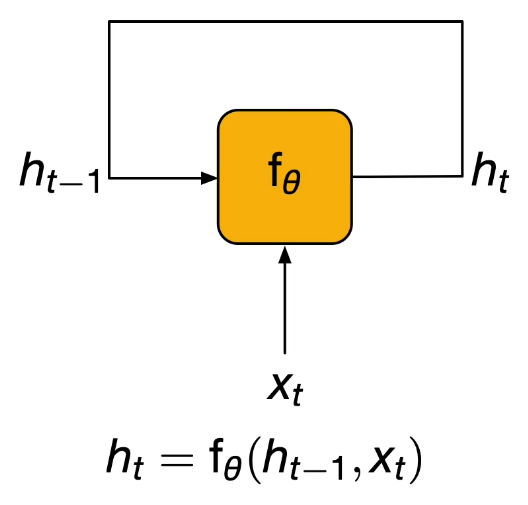
This is expressed as $f_{\theta}$ where $h_t = f_{\theta}(h_{t-1}, x_t)$.
When people talk about RNNs they normally mean this model. However, some people in the literature mean any network that is not a DAG when it comes to inputs/outputs.
These networks present a problem when running backpropagation — as the training data is sequences of words, but the network uses this state variable. However, to carry out backpropagation we just ‘unroll’ the network. E.g.
$$ f_{\theta}(x_1 x_2 \ldots x_n) = f_{\theta}(x_n, f_{\theta}(x_{n-1}, f_{\theta}(x_{n-2}, \ldots f_{\theta}(x_1, 0)))) $$For very long inputs this can make backpropagation very long — so sometimes we use ’truncated backpropagation through time’, where we instead only backpropagate for a fixed number of time steps and cut it short at that point.
RNNs are ’two-headed’ — they have a forward mode which is only about updating the hidden state $h_t$, but they can also be used to output $y_t$. The output $y_t$ depends on the hidden state $h_t$ and can be calculated at all steps or only a given one. It is usual that we run the model in ‘forward mode’ through the whole input and only call the output at the end.
This is the simplest RNN model, where we use an affine combination of the input vectors with a bias term and an activation function to generate another state.
$$ h_t = f_{\theta}(h_{t-1}, x_t) = \sigma_{\theta}(U_{\theta} x_t + V_{\theta} h_{t-1} + a_{\theta}) $$To get the output of the network we apply another transformation.
$$ y_t = \sigma_{\text{out}}(W_{\text{out}} h_t + \beta_{\text{out}}) $$Where the activation functions are typically logistic functions or tanh.
The gradient presents an issue due to the vanishing/exploding gradient problem. That is, as the sequence length increases, the gradient either vanishes to zero or explodes to infinity. For example, consider a simple update function
$$f_{\theta}(x_t, h_{t-1}) = W_{\theta}(x_t + h_{t-1})$$When considering the derivative
$$\frac{\partial h_t}{\partial x_0} = W_{\theta}^t$$Now if $|W_{\theta}| > 1$ the gradient diverges, whereas if $|W_{\theta}| < 1$ it converges to zero.
# Long short-term memory
A model was proposed to get around the issue of the vanishing/exploding gradient problem. This was called the long short-term memory model — which can train itself to forget information in the past. Here we introduce 5 new terms:
Forget gate $f_t$: This is a gate that decides what to forget.
Input gate $i_t$: This is a gate that decides what to input.
Candidate update $u_t$: This is the update that is used to update the state.
Output gate $o_t$: This is a gate that decides what to output.
Cell state $c_t$: This is the state of the cell.
These gates are all calculated using:
$$ \begin{bmatrix} f_t \\ i_t \\ u_t \\ o_t \end{bmatrix} = \begin{bmatrix} \sigma \\ \sigma \\ \tanh \\ \sigma \end{bmatrix}(\begin{bmatrix} W_{f} \\ W_{i} \\ W_{u} \\ W_{o} \end{bmatrix} \left ( W_{\theta} \begin{bmatrix} x_t \\ h_{t-1} \\ \end{bmatrix} + b_{\theta} \right ) $$(Note here that $\sigma$ is the sigmoid function.) These are then used to update the cell state $c_t$ and hidden state $h_t$ as follows:
$$ \begin{aligned} c_t &= f_t c_{t-1} + i_t u_t \\ h_t &= o_t \tanh(c_t) \end{aligned} $$# Tokens
Rather than splitting text into words, modern language models operate on tokens — subword chunks derived from the training corpus. The standard algorithm is Byte Pair Encoding (BPE): start with individual characters, then iteratively merge the most frequent adjacent pair into a single token, repeating until a target vocabulary size is reached. The result is that common words become single tokens, while rare or unknown words are decomposed into subword pieces.
This is preferable to words for several reasons:
- Compression: tokens are chosen to minimise the total number of units needed to represent the corpus, giving better information-theoretic efficiency than a fixed word vocabulary.
- Unknown words: a word vocabulary has no representation for words outside it. Tokens always fall back gracefully — ultimately to individual bytes.
- No alphabet needed: modern tokenisers operate on the 256 possible byte values rather than Unicode characters or words. This means any sequence of bytes — any language, punctuation, code, or binary data — can be represented without ever producing an unknown token.
The vocabulary size (typically 50k–100k tokens) is a trade-off: larger vocabularies mean fewer tokens per sequence (cheaper attention) but a bigger embedding table and output softmax.
Tokens do not respect word boundaries. "token" and " token" (with a leading space) are typically different tokens.
This is why LLMs struggle with character-level tasks like counting letters — the model never sees individual characters, only tokens, and must reason about their internal structure.
# RNNs as language models
First, to go from words to something a model will understand, we take a one-hot embedding of our tokens. This means we pick an underlying vocabulary $W$ and then embed a particular token as a unit vector with a single non-zero entry.
Now a sequence of words can be represented as a sequence of vectors. We can use these as inputs to our RNN. Note that we can now use the model in forward mode along our sequence before we get it to output the prediction of the next word in the sequence.
# Evaluation
It is common in machine learning to use cross-entropy for our loss function. Suppose we have two probability distributions $p, p^{\ast}$ over the state space $\mathcal{X}$; then this is defined as:
$$ H(p^{\ast}, p) = -\sum_{x \in \mathcal{X}} p^{\ast}(x) \log p(x) $$In the NLP setting we can extend this to the ‘per-word cross-entropy’:
$$ H(s) = - \frac{1}{N} \sum_{i=1}^N \log p(w_i \vert w_{i-1}, \ldots ) $$This is commonly used as a loss function for language models. Another quantity that could be used for this is the perplexity:
$$ \begin{aligned} \text{Perplexity}(s) &= \prod_{i=1}^N \sqrt[N]{\frac{1}{\mathbb{P}(w_i \vert w_{i-1}, \ldots)}}\\ &= b^{-\frac{1}{N} \sum_{i=1}^N \log_b \mathbb{P}(w_i \vert w_{i-1}, \ldots)}\\ &= b^{H(s)} \end{aligned} $$This is tied to per-word cross-entropy as laid out above. The lower the perplexity the better.
# Training
To train a RNN language model, we use the input data but run it both in forward and output mode. Then we can compare the output of each step to the next word to get the loss (after applying softmax). Then the loss of the whole model is simply the average loss across the whole text.
# Transformer encoder
A transformer encoder is an alternative to the RNN for producing contextualised representations of a sequence. Rather than processing tokens one at a time and compressing history into a hidden state, it processes all tokens simultaneously using self-attention — i.e., the non-local layer idea from week 8 applied to the full sequence.
For an input sequence of $n$ token embeddings $X \in \mathbb{R}^{n \times d}$, each layer computes:
$$ \text{Attention}(Q, K, V) = \text{softmax}\!\left(\frac{QK^T}{\sqrt{d_k}}\right)V, \quad Q = XW_Q,\ K = XW_K,\ V = XW_V $$Each token attends directly to every other token, so there is no sequential bottleneck and no vanishing gradient over long distances. This also means the computation is fully parallelisable across the sequence — a major practical advantage over RNNs (which must process tokens sequentially).
Since attention is order-agnostic, positional encodings are added to the token embeddings to inject sequence order. These can be fixed (sinusoidal) or learned, and they determine the model’s context window — the maximum sequence length $n$ the model was trained with. Extending beyond this degrades performance because the model has never seen those positions.
| RNN | Transformer encoder | |
|---|---|---|
| Neighborhood | Previous hidden state only | All tokens (via attention) |
| Long-range dependencies | Hard (vanishing gradient) | Direct — O(1) path between any two tokens |
| Parallelism | Sequential | Fully parallel |
| State | Fixed-size hidden vector | Full sequence of vectors |
# Masked language models
We can use a transformer to learn ‘ideas’ about the language. One technique is masked language modelling, where we mask certain tokens and get the model to predict what each masked token is. For it to be able to do this, we add to each input token a positional encoding indicating its position within the sequence. Whilst this task in itself is not useful, we can still use the learning this model has done for other tasks using transfer learning.
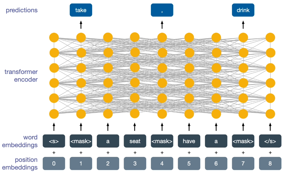
There are a couple of interesting tasks we can transfer this model to doing:
Token-level tasks: Predicting what each token is — for example, whether it is a date, location, or person’s name.
Cross-lingual tasks: Translating between languages.
Natural language inference: Given a premise and a hypothesis, predict whether the hypothesis is entailed by, contradicts, or is neutral with respect to the premise.
These models tend to be massive in size. This means they can be very expensive to train and run — however, we can ‘pass their knowledge on’ to smaller models using a teacher-student approach. Here we use the predictions of the teacher to act as the loss function for the student. This technique is called ‘knowledge distillation’ and works very well, but it is still an open research question as to why.
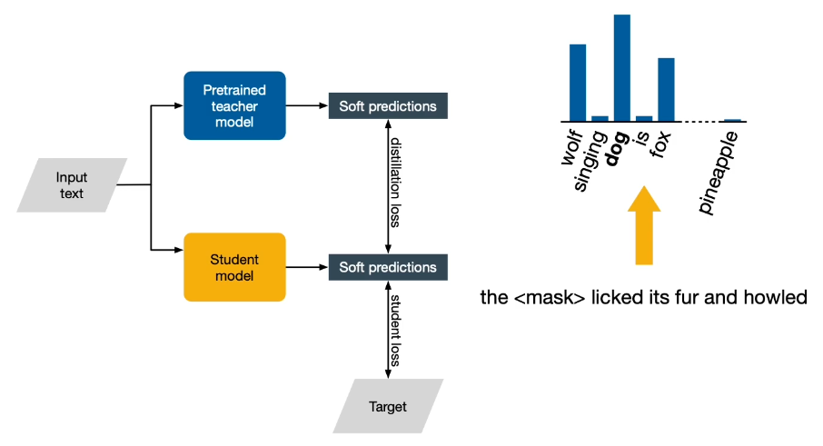
One explanation for why this is so powerful is that the teacher not only communicates the correct answer, but also passes on its probability distributions over other similar words.