Up to now we have been doing image classification. However, there are lots of other tasks that we can do with images:

• Semantic segmentation: Associate a class distribution per pixel.

• Instance segmentation: Class distribution per pixel where we differentiate different objects, i.e. associate a unique ID.

• Object detection: Create a list of bounding boxes for objects in the picture with a class distribution per box.

# Segmentation

In the previous lectures we studied CNNs. These normally involve multiple convolutional and pooling layers that reduce the image into a feature vector. This in turn was fed into fully connected layers to output class probabilities.

For segmentation problems we want an output per pixel. So we need an output:

1. Must maintain spatial information.

2. Must have output size the same as the input.

This is exactly what the fully connected layers throw away.

# Fully convolutional hidden layers

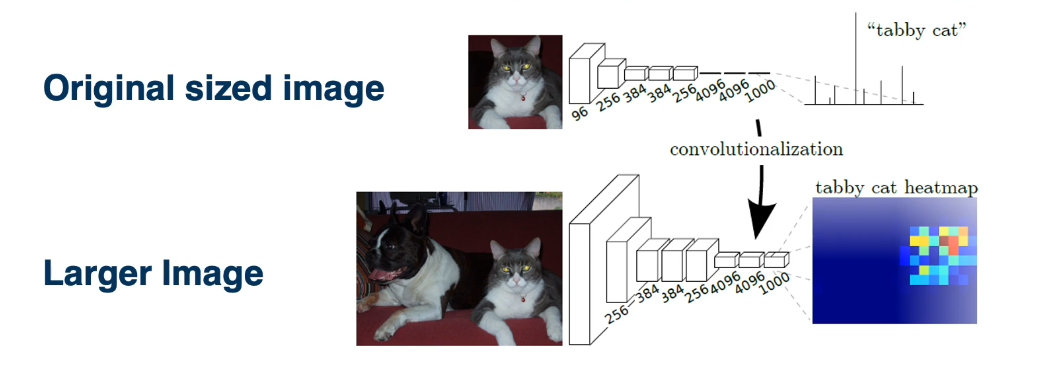
The core idea here is to replace fully connected layers with convolutional kernels that span the entire spatial input. Since the kernel covers the full input, each application produces a single scalar — equivalent to Wx + b for a fixed-size input, with one kernel per output node. However, framing it as a convolution means the same kernel can slide over a larger input, producing a spatial output map rather than a single scalar — enabling per-pixel predictions.

A practical application of this is training a classifier on smaller images, then running it on larger images. The kernels slide across the larger input and produce a heat map indicating where in the image each class is likely to appear. The spatial resolution of this output is slightly lower than the original input due to downsampling in the network, but this is an acceptable trade-off.

# Encoder-decoder architectures

Another approach is to carry out the ‘inverse’ to the convolutional layers. If we call the classic CNN the ’encoder’ we define the opposite notion of the ‘decoder’ that works in reverse.

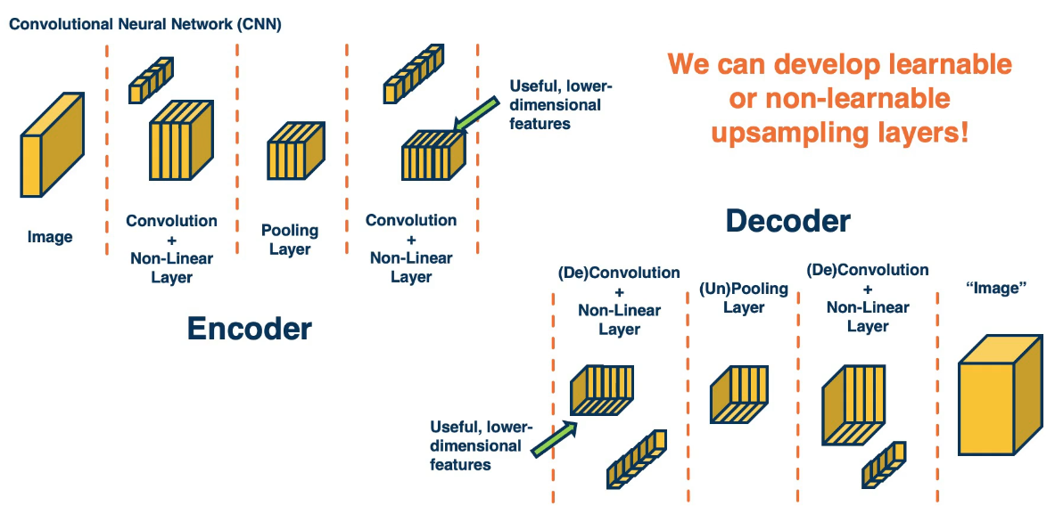
This has two main blocks:

• (De)convolutional layers that produce a spatial output map.

• (Un)pooling layers that unpack a single scalar into a bigger image.

The max unpooling layer above does not have any learnable parameters and uses values from the encoder stage to operate. However for the de-convolutional layers it might be advantageous to have learnable parameters.

We can use transfer learning here to train the encoder network on a big dataset such as ImageNet but then jointly train the encoder/decoder on our hand labelled data.

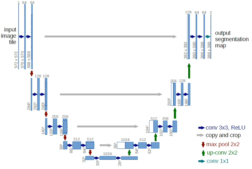
We can also use the ideas such as skip connections to help data flow between the encoder and decoder such as U-net below.

# Object detection

Object detection similar to segmentation has to output multiple results. However, unlike segmentation the number of boxes is not fixed at the beginning. There are multiple approaches to this, as we explore below.

# Fully convolutional networks

The first approach is to use fully convolutional networks like above. Here we use a multi-headed network predicting 5 things:

• The (x,y) coordinates of the box.

• The width and height of the box.

• The class probability for the box.

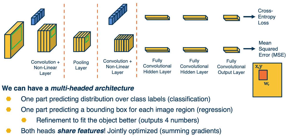
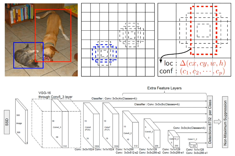
We can do this at multiple scales as well - to get a larger mix of detections. This can be further improved using:

• Decrease subsampling ratio: This allows us to increase the resolution of the output.

• Non-maximal suppression: This allows us to remove overlapping boxes.

# Single shot Detector (SSD)

Similar to above, but this combines the rescaling tricks into a single network. This at each point assigns multiple boxes (that can be tuned using a hyperparameter). There are multiple tricks such as skip layers and decrease subsampling ratios that help us get this in one.

# You Only Look Once (YOLO)

This is a similar idea as SSD but only uses one resolution.

# Evaluation

To compare these algorithms we use COCO which is similar to ImageNet but with multiple objects per image. However, to work out how good a match is for a particular bounding box is a little more complicated. Here we normally use Mean Average Precision (mAP).

1. For each bounding box, calculate intersection over union (IoU) between the predicted box and the ground truth box:

IoU ranges from 0 (no overlap) to 1 (perfect overlap).

2. Keep only those with IoU greater than some threshold (e.g. 0.5).

3. Sort remaining detections by classification confidence, then calculate precision and recall at each threshold:

Where TP is the number of true positives, FP is the number of false positives, and FN is the number of false negatives.

4. Calculate average precision $\text{AP}_i$ for this IoU threshold $i$ as the area under the precision-recall curve:

where $P(n)$ is precision and $\Delta R(n)$ is the change in recall at the $n$th confidence threshold. Steps 2–4 are repeated for each IoU threshold $i$.

5. Average over all IoU thresholds to get mean Average Precision:

# R-CNN

The idea behind R-CNN is to use a two stage network to:

1. Find regions of interest (ROI) with object-like things.

2. Classify those regions using a scaled version of the ROI.

Finding ROIs is an old problem and has lots of unsupervised learning approaches that handle this - such as Selective Search. The trouble with these approaches is that they output thousands of bounding boxes. This also takes a long time - such as 1 second per image.

# Fast R-CNN

A computational issue with the above algorithm is that with thousands of crops, you need to essentially recalculate a classifier on multiple images that might have massive overlap. In other words, you are redoing a lot of the computation repeatedly. So we could instead push the whole image through the CNN first - then pick the regions of the feature map that relate to each ROI.

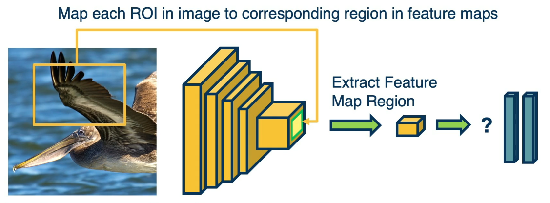
This has a problem though as each ROI might return different sizes within the feature map. So we use a technique called ROI pooling. For each ROI grid we run a max pool over a correctly sized region to output the correct sized feature map.

We can now backpropagate all the way through this and train the features as well as the classifier. (Notice we can do this even through the ROI pooling as we can control how we update the gradients using the max pool.)

# Faster R-CNN

Fast R-CNN uses a secondary algorithm to find the ROIs. It would be nice to incorporate this into a single network so we can co-learn the classifier with the ROI generator. To do this we add the Region proposal network (RPN) that uses the same feature maps. Then the RPN outputs an objectness score and bounding box. Then we select the top $k$ objects for classification.

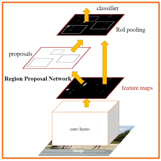
Here we have an issue where some parts of the RPN are not differentiable as there is no clear meaning of what happens when you change the bounding box dimensions. Therefore this is often trained in a two stage fashion.

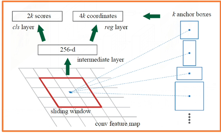
Similar to YOLO, we have the issue of needing different sizes and scales for the ROI boxes. So we use a similar technique where in each point in the box we have multiple anchor boxes of different sizes. That means we get lots of output scores for each anchor box at each location.

# Mask R-CNN

There are multiple variants of this algorithm, such as Mask R-CNN, which not only outputs boxes and classes but also masks indicating which pixels belong to each object.