When working with visual data you can visualise how the network is making decisions. This allows insight into why it makes decisions. There are different ways to do this:

• Weights: For simple linear classifiers, you can plot the weights for different class outcomes and reshape them into an image. This gives you a mask you can visualise to see how it views the object. For convolutional neural networks you can do the same for the kernels to see what features they are picking out.

• Activations: For CNN layers you can look at the output images after applying the kernel to the image. These can be put into gray scale and still should represent the image fairly closely.

• Gradients: For a particular image you can push the gradient all the way back to the image itself, this allows you to visualise this gradient overlayed on the image itself. This gives you insight into what the network thinks is important.

• Robustness: These techniques allow you to enrich your data set with more examples. As you change images along the gradients to get closer to different classifications.

# Weights

For visualising weights, you normally need to rescale them to be between 0 and 255. This can be done on layers that connect back to the image themselves but is not always possible — for example in CNNs the fully connected layer doesn’t connect to the image itself.

You can also visualise the CNN kernels themselves. This works well for older networks like AlexNet where they are pretty large (11×11) but nowadays with 3×3 layers this is less informative.

# Output maps

Instead of visualising the kernels themselves - you can find all the images in your dataset that cause it to have the largest value. This should relate to what ‘features’ or commonalities it is trying to pick out.

# Dimension reduction

There are techniques like t-SNE that allow you to plot your data on a 2D plane where it preserves the distances in the classifications. These visualisations provide a nice way to see how your data is clustered. People also use principal component analysis (PCA) for this as well — but t-SNE is a more advanced technique.

# Gradient based methods

The core technique for gradient based methods is to put an image through the forward pass of the network. Then you can backpropagate changes all the way back to the image itself. For example, calculating:

$$ \frac{\partial s}{\partial x} $$

(Here $s$ is the score before the softmax layer. This is done because taking the softmax and loss function can add complexity to what the gradients are actually showing you.) This tells us how to change the image so that it is closer to a given class. Though we can actually use the same idea to see what the layers in between are doing as well. We can look at gradients such as:

$$ \frac{\partial h_i}{\partial x} $$

This tells us how the image will need to change to increase or decrease a value within $h_i$ which gives us a sense of what that neuron relates to. These are called ‘saliency maps’.

You can use these ‘saliency maps’ to see what ‘bit’ of an image is triggering that classification. This is powerful as it lets you find out not only what the network thinks it is classifying but which bit of the image is causing that classification. This means we ‘for free’ get object localisation as well as classification.

You can use this technique to debug networks as well. For example, if in your training set all of one class has a strongly correlated feature then you may cause misclassifications in your test set if other classes have that correlated feature as well. For example, if all your pictures of wolves are in snow - you can see the wolf classifiers gradient pick out snow instead of the wolf itself. This tells you your network has learnt the wrong thing and you need to get better training data.

How you do this can be complicated. Sometimes you don’t want to propagate the negative part of the gradient so you can choose to zero this out as well as the bits of the map that get zeroed from ReLU. This is called ‘guided backpropagation’ and is normally used for this process.

# Grad-CAM

Rather than propagating gradients all the way back to the input pixels (like saliency maps do), Grad-CAM stops at the last convolutional layer. By this point the network has built up high-level semantic features (shapes, textures, object parts), so the activations there are spatially meaningful.

The key insight is: instead of asking “which pixels should change?”, Grad-CAM asks “which feature maps in the last conv layer matter most for this class, and where are they active?”

The steps are:

1. Compute gradients of the class score $y^c$ w.r.t. each feature map $A^k$ in the last conv layer:

   $$\frac{\partial y^c}{\partial A^k}$$

2. Global Average Pool those gradients spatially — collapsing each feature map’s gradients into a single importance weight $\alpha_k^c$ (where $Z = H \times W$ is the number of spatial positions in the feature map):

   $$\alpha_k^c = \frac{1}{Z} \sum_{i,j} \frac{\partial y^c}{\partial A^k_{ij}}$$

3. Weighted sum + ReLU to produce the final heatmap:

   $$L^c = \text{ReLU}\left(\sum_k \alpha_k^c A^k\right)$$

The ReLU discards feature maps that hurt the class score, keeping only regions that positively contributed.

	Saliency Maps	Grad-CAM
Gradient w.r.t.	Input pixels	Last conv layer activations
Resolution	Full image (fine, noisy)	Feature map size (coarse, clean)
Class-discriminative	No	Yes — different classes give different heatmaps
What it shows	Which pixels are sensitive	Where in the image the class is located

This means Grad-CAM gives you object localisation essentially “for free” from a classifier — the same benefit noted above for saliency maps, but with a cleaner and more class-specific signal.

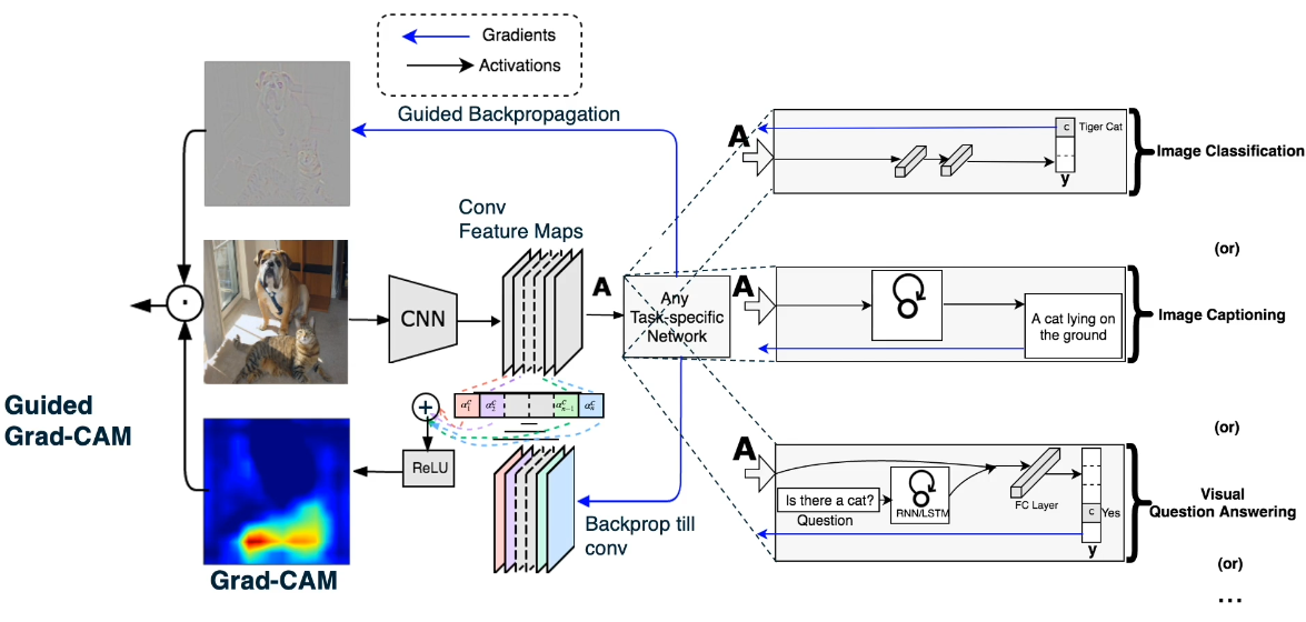
If used for question-answering tasks — for example “What animal is in this picture?” — you can use Grad-CAM to see what the network is ’looking at’ when it makes its decision. This has been shown to be very powerful as if images contain multiple animals you can see what bit the network is focusing in on when it answers.

# Optimising images

You can use the gradients from the saliency maps to ‘change’ your image to more closely align with a specific class. For example, you could take an image of a dog and move it in the direction of ’elephant’ - to generate a new image. This allows you to either:

• Generate new images starting from random noise.

• Harden the network by generating new examples labeled correctly.

This is essentially gradient ascent on the image itself for a particular class. We can here also apply regularisation preferring smaller changes in the pixel values so as to prefer images that are similar to the previous image.

When using this technique for hardening you can quickly work out that very small changes to the input image can dramatically throw the classification off. In the extreme case you can get ‘single pixel attacks’ where you change one pixel in the image to get a completely different classification. This is a good technique to harden images to adversarial attacks against your classification.

However, this is a cat and mouse game to make networks robust. It is an active area of research on how to make these attacks and how to defend from them. These range from ‘white-box attacks’ like using gradient ascent to ‘black-box attacks’ where you just get the output of the model.

# Other robustness techniques

There are other ways to observe how robust your network is. For example, you can blur or change the lighting of your image and see how stable the scoring is. An interesting result here is networks trained on ImageNet have an inverse relationship between accuracy and robustness. In other words, more modern networks which are more accurate tend to be less robust on the classes they solve for. This indicates their decision boundaries are much finer and could indicate overly fitting the problem. In comparison, AlexNet is relatively robust.

Another technique is to look at biases within the network. For example you can see if the network prefers shape or texture by combining two different images shape and texture and seeing which classification wins out.

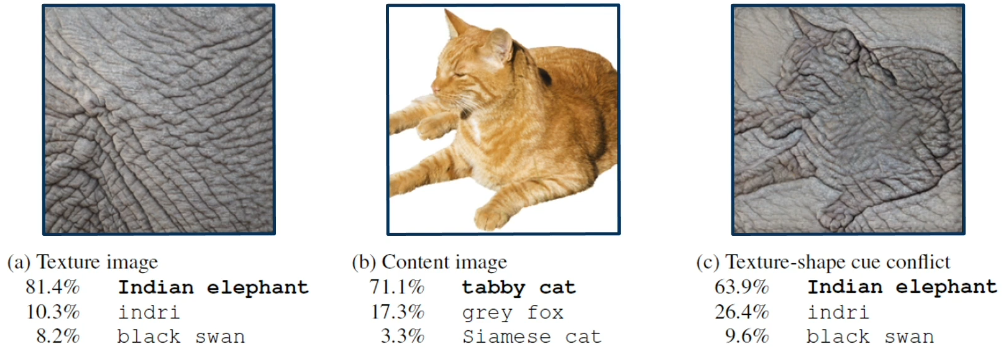
Here you see that all the imagenet classifiers are much more biased towards texture rather than shape. But again this bias is much larger in more accurate networks.

# Style transfer: Gram matrix

Suppose now we would like to change an image so that it is in a different style. For example, change a picture of a dog so that it looks more like a painting than a photo.

We can use CNN networks to do this. The base idea comes from creating a new loss function based on the layers of the CNN network.

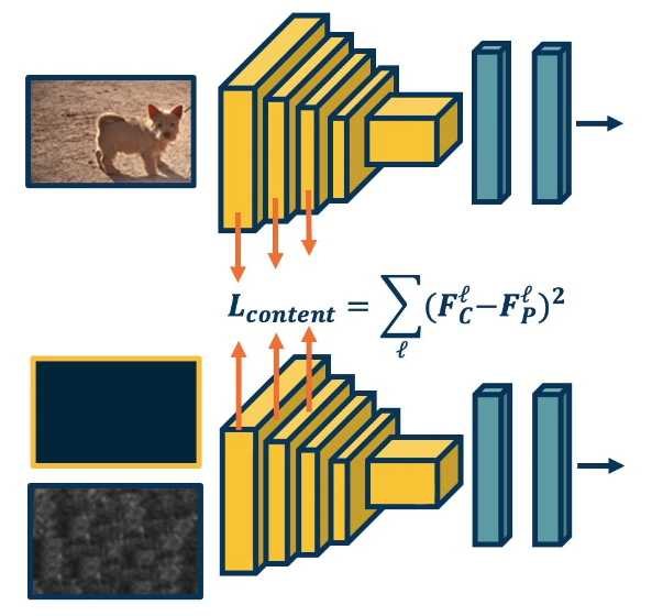
Here we put the image of a dog through a trained network. We also put a blank image through the network. At each layer of the network we can define a ’layer-based’ loss function which is just the position wise difference squared between the feature map of the dog vs the empty image. This can now be our loss function and we can run gradient descent on the blank image using this loss function. This way we can change a blank image to be more like a dog over time.

The technique above will make the image more like a dog but to add in a new style we can do the same trick but with a different image.

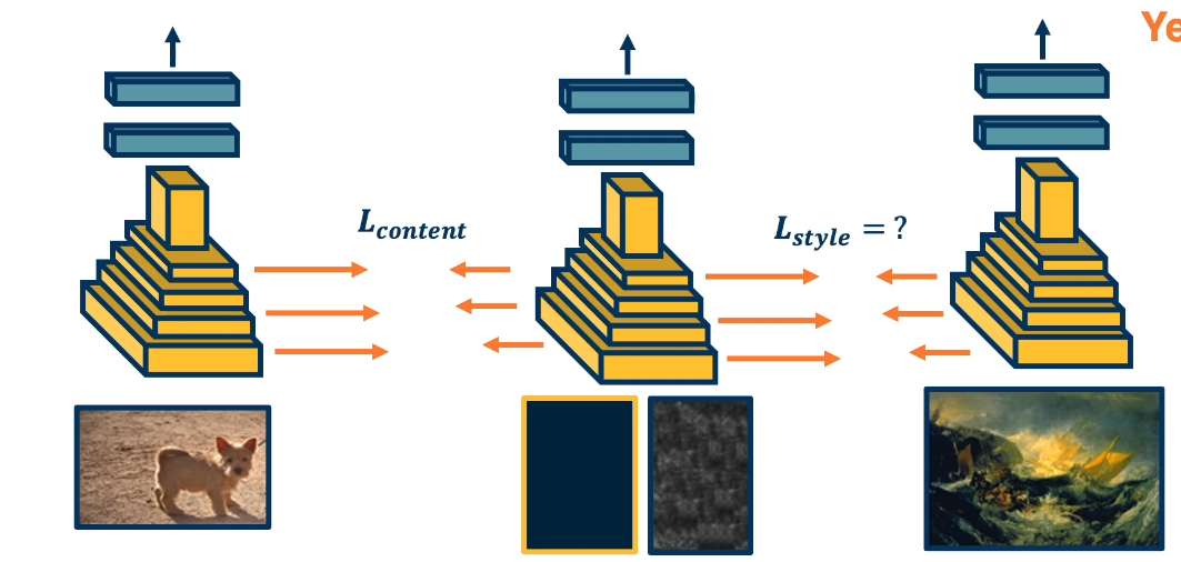
However, for the style image we don’t want spatial information — we only want its texture and patterns. The key idea is to use correlations between feature maps rather than the feature map values themselves. Correlations tell you which filters tend to activate together across the image, which captures texture (e.g. “brushstroke-like edges and warm colours co-occur”) without encoding where anything is.

# Gram matrix

For a given layer $l$ with $N_l$ filters and $M_l$ spatial positions, we flatten each filter’s activation into a vector and take pairwise inner products. This gives the Gram matrix $G^l$, an $N_l \times N_l$ matrix:

$$G^l_{ij} = \frac{1}{M_l} \sum_k F^l_{ik} \cdot F^l_{jk}$$

where $F^l_{ik}$ is the activation of filter $i$ at spatial position $k$. Each entry $G^l_{ij}$ measures how correlated filter $i$ and filter $j$ are across the whole image — summing over all positions throws away the “where” and keeps only the “what co-activates with what”.

The style loss is then the squared difference between the Gram matrices of the style image $S$ and the generated image $X$, summed across multiple layers:

$$L_\text{style} = \sum_l w_l \sum_{i,j} \left(G^l_{ij}(S) - G^l_{ij}(X)\right)^2$$

Using multiple layers captures style at different scales — early layers encode fine textures, deeper layers encode broader patterns.

# Combined loss

The total loss is a weighted sum of content and style losses:

$$L_\text{total} = \alpha \, L_\text{content} + (1 - \alpha) \, L_\text{style}$$

Gradient descent on the generated image $X$ then simultaneously pulls it toward the content of the dog image and the style of the painting.