In this week, we will focus on how to calculate the backward pass for convolutional neural networks and then talk about how they are practically used.

# Backward pass

Remember that the definition of a CNN for a kernel $K$ of size $K_1 \times K_2$ going from input $i$ to output $O$ is:

$$ O(x,y) = K \ast I(x,y) = \sum_{i=0}^{K_1 - 1} \sum_{j=0}^{K_2 - 1} I(x + i,y + j)K(i,j) $$

Then let’s calculate

$$ \begin{aligned} \frac{\partial L}{\partial K(a,b)} = & \sum_{x = 0}^{H - K_1} \sum_{y=0}^{W - K_2} \frac{\partial L}{\partial O(x,y)} \frac{\partial O(x,y)}{\partial K(a,b)}\\ = & \sum_{x = 0}^{H - K_1} \sum_{y=0}^{W - K_2} \frac{\partial L}{\partial O(x,y)} \frac{\partial}{\partial K(a,b)} \sum_{i=0}^{K_1 - 1} \sum_{j=0}^{K_2 - 1} I(x + i,y + j)K(i,j) \\ = & \sum_{x = 0}^{H - K_1} \sum_{y=0}^{W - K_2} \frac{\partial L}{\partial O(x,y)} I(x + a,y + b) \\ = & \left(\frac{\partial L}{\partial O} \ast I\right)(a,b) \\ \end{aligned} $$

This gives us that the backward pass is also a convolution operation between the previous derivative and the input.

Though to continue passing the gradient backward we need:

$$ \begin{aligned} \frac{\partial L}{\partial I(a,b)} & = \sum_{x=a+1-K_1}^{a} \sum_{y=b+1-K_2}^{b} \frac{\partial L}{\partial O(x,y)} \frac{\partial O(x,y)}{\partial I(a,b)}\\ & = \sum_{x'=0}^{K_1 - 1} \sum_{y'=0}^{K_2 - 1} \frac{\partial L}{\partial O(a - x',b - y')} \frac{\partial O(a - x',b - y')}{\partial I(a,b)}\\ & = \sum_{x'=0}^{K_1 - 1} \sum_{y'=0}^{K_2 - 1} \frac{\partial L}{\partial O(a - x',b - y')} \frac{\partial}{\partial I(a,b)} \sum_{i=0}^{K_1 - 1} \sum_{j=0}^{K_2 - 1} I(a - x' + i,b - y' + j)K(i,j)\\ & = \sum_{x'=0}^{K_1 - 1} \sum_{y'=0}^{K_2 - 1} \frac{\partial L}{\partial O(a - x',b - y')} K(x',y')\\ & = \left(\frac{\partial L}{\partial O} \star K\right)(a,b) \end{aligned} $$

Here $\star$ denotes cross-correlation (no kernel flip), while $\ast$ denotes convolution (kernel flipped), recovering the duality between the two operations.

Computationally, both of these operations are performed by the im2col operation. Which can be implemented efficiently on the GPU and in standard ML packages.

# Structure of a CNN

We normally stack convolutional and pooling layers together to perform hierarchical feature extraction.

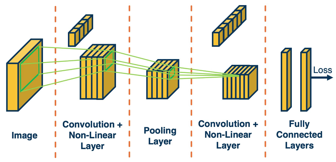
Even when using small convolution layers such as 3x3 stacking them means that features towards the end still use most if not all of the image for the final value. These techniques have been around since the 1980s which used the below network to perform character recognition.

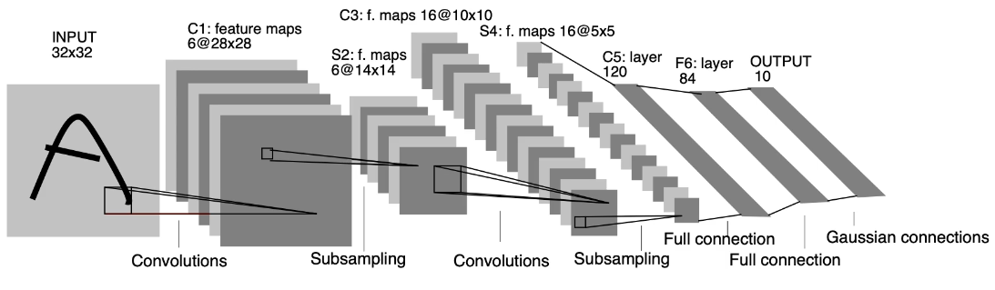
You will see here and later that it is common for CNNs to slowly decrease the size of the image whilst increasing the number of features extracted. This is common and was continued later as well.

A big turning point for CNNs was their performance in ImageNet (a problem of classifying 1 million images into 1000 categories). When the first CNN, ‘AlexNet’, was used it reduced the top-5 error from ~26% for the best prior network to ~15%, a dramatic improvement that sparked the deep learning era.

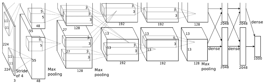
This was split into two due to memory constraints within their hardware at the time. They also used larger CNNs with size 11 and 5 at the start and larger strides. This was shown to not be hugely efficient - so faded out over time - with most networks now using 3x3 convolutions with a stride of 1. They also used Local Response Normalisation (LRN) layers within their CNN, but these were later superseded by Batch Normalisation (Ioffe & Szegedy, 2015) and have since been dropped from most architectures. However, one of the large improvements was the use of ReLU over sigmoid - which as we talked about before increased the amount of gradient flow through the network. They also used dropout layers to prevent overfitting.

Later attempts that improved efficiency are for example VGG.

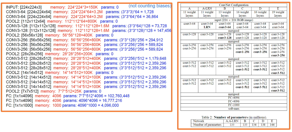
Notice here how they use ‘modules’ of CNN layers and compose them.

However, here we see an interesting duality. The CNN layers use a lot more memory - for calculating gradients we need to store the values at each layer. However, the CNN layers don’t use that many variables as they share values. In contrast, the fully connected layers that perform classification don’t use up much memory but have a lot of variables.

To get better and better performance researchers started adding in more and more layers increasing the number of parameters. However, they noticed at some point they would not get an increase in performance. This was later overcome by adding in residual blocks and skip connections. These are layers that augment the values a little bit rather than fully change it.

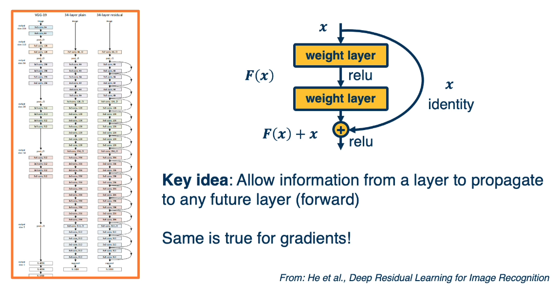
This was shown to increase the gradient flow through the larger and larger networks which allowed it to train the parameters more efficiently.

Now we are starting to look in the opposite direction. How can we get the same performance using less parameters? There is an area of active study here where they try to optimise the architecture to need fewer layers.

# Transfer learning/generalisation

There are multiple sources of error in ML:

• Model error: The error induced by your model not being expressive enough to reflect the reality of the situation.

• Optimisation error: The error induced by the optimisation process not being able to find the global minimum.

• Estimation error: The error induced by the difference in your test data vs reality. For example, you model over fitting or not containing enough data on certain classes.

We normally get payoffs between these different types of errors. For example, more complicated models may have a smaller Model error but then may increase the optimisation error. Or if we have increased the number of parameters the amount of data is insufficient and we get a larger Estimation error.

In fact, normally data is the largest limiting factor in most real world problems. Therefore, transfer learning has become fairly common. This is as follows:

1. Take a trained model on a similar domain - such as ImageNet.

2. Remove the last layer where we go to our classes.

3. Retrain our network using our data — either updating only the last layer’s weights (feature extraction) or fine-tuning all layers with a small learning rate.

This then uses all the hard work put in on a rich dataset and applies it to our use case. This has amazing performance beating out custom work on a lot of problems.

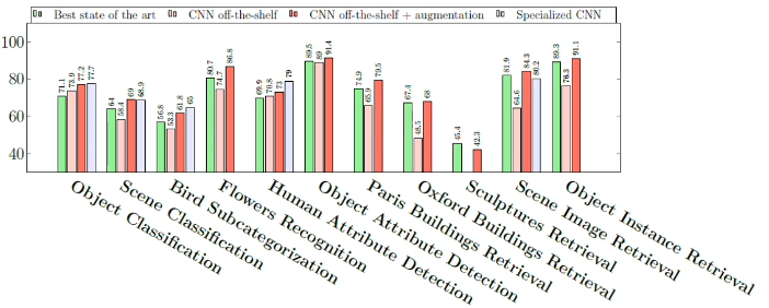
This can even transfer across domain from image recognition to object tracking. However, there are certain cases where it will not work well:

1. Where the source and target domain are very different e.g. photographs to sketches.

2. When you don’t have enough data in the target domain so you can’t train the weights well.

# Limits

When working on any dataset there will be some irreducible error. However, progress normally follows a power law with the more data we give it.

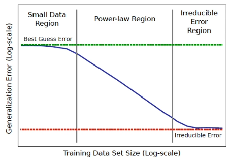
Some Google researchers showed however that for ImageNet we are still not at the point of hitting the irreducible error. Showing that with more data we can still get better performance.

There is also research in the opposite direction, working out how with little data we can increase transferability within problems.