Previously, we have investigated supervised learning where we want to estimate $\mathbb{P}(y \vert x)$ i.e. the probability of a label given some input. Next we will look at unsupervised learning where instead we just want to look at $\mathbb{P}(x)$ i.e. the distribution of inputs. This is a complex way to say - instead of labeling some data we want to generate a sample from it. For example, given lots of pictures of cats — can you generate a new picture of a cat? This is actually a hard task to do.

Lots of the methods to do this fix the model and use log likelihoods e.g. once we parameterise our model using parameters $\theta$ we look for:

$$ \begin{align*} \theta^{\ast} = & \argmax_{\theta} \prod_{i=1}^m p_{model} \left( x^{(i)} ; \theta \right)\\ = & \argmax_{\theta} \log \prod_{i=1}^m p_{model}(x^{(i)} ; \theta) = & \argmax_{\theta} \sum_{i=1}^m \log p_{model}(x^{(i)} ; \theta) \end{align*} $$

The one strange thing about this output is given you have a fixed model with fixed parameters when you are generating a picture of a cat - won’t it always be the same? The answer is no - instead we start with a small amount of random noise to feed into the model. Often this is a vector of gaussian noise with mean 0 and variance 1.

Generative models is a broad field with many different approaches - below we will focus on three of them.

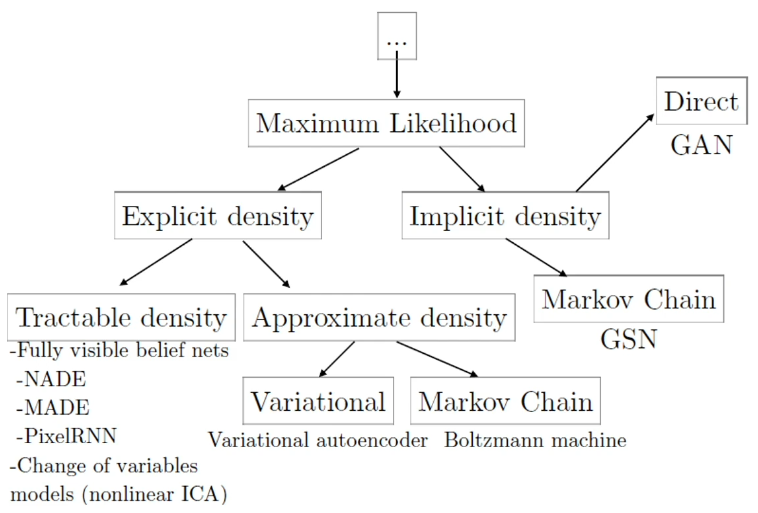
# PixelRNN / PixelCNN

The first approach is to treat the whole picture as a conditional distribution. This goes pixel by pixel in its generation breaking down the computation as follows:

$$ p(x) = \prod_{i=1}^{n\times m} p(x^{(i)} | x^{(i-1)}, x^{(i-2)}, \dots, x^{(1)}) $$

Functionally this works by choosing an ordering of the pixels then generating new pixels based on the old ones.

This then fits perfectly into the NLP models we worked on before where our sequence is pixels instead of words. This allows us to train using teacher forcing and apply maximum likelihoods but it is slow to generate and can only consider a few pixel context to vary the image.

Another approach is to use a CNN which is trained on masked data to give predictions of missing pixels. This speeds up the training as we can easily generate a lot of data but still has a slow generation process.

This also enables ‘filling in’ space/background of images if it was missing.

Fundamentally these approaches are limited by the context they can take in. This means whilst they can ‘on the whole’ look realistic in the finer details they normally don’t look right.

# Generative Adversarial Networks (GANs)

The main idea in GANs is instead of training a single network to try and output images from the distribution of $x$. Instead we train two models - one will be trained to output images from $x$, the other will be trained to predict fake/real images on the output of the first model and our real images. This sets up a game dynamic where one model improving improves the other and vice versa.

Functionally this works by first generating a vector of random values $N(0,1)$ then we feed this through a neural network (normally a CNN decoder) to output our image. This network is called the generator. Then we take a batch of these images and some real images and feed it through another neural network. This network is called the discriminator. Then we define the loss of the second network based on if it guessed the real/fake correctly. Then invert this loss to train the first network.

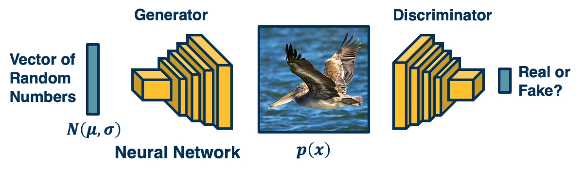
Given our generator $G$ where $G(z)$ is an image and discriminator $D$ where $D(x)$ is a probability $[0,1]$ of being a real image the minimax objective can be stated as follows:

$$ \min_{G} \max_{D} V(D,G) = \mathbb{E}_{x \sim p_{data}} [\log (D(x)) ] + \mathbb{E}_{z \sim N(0,1)^n}[\log(1 - D(G(z))) ] $$

The first term is log likelihood of $D$ saying the real image is real. The second term is the log likelihood of the $D$ saying the generated images are fake. This then defines our two loss functions with the discriminator getting both the real and fake images as input:

$$ \nabla_{\theta} \frac{1}{m} \sum_{i=1}^m \left [ \log D(x^{(i)}) + \log \left ( 1 - D ( G ( z^{(i)})) \right ) \right ] $$

Whereas the generator only gets the results of the fake images.

$$ \nabla_{\theta} \frac{1}{m} \sum_{i=1}^m \log (1 - D(G(z^{(i)}))) $$

This turns out to be a bad loss function from the generator’s perspective.

• High gradient when $D(G(z))$ is high (that is when the discriminator is wrong).

• Low gradient when $D(G(z))$ is low (that is when the discriminator is right).

This is backwards from what the generator needs: low gradient signal when it is losing (discriminator is right, $D(G(z)) \approx 0$) and high gradient signal when it is already winning (discriminator is fooled, $D(G(z)) \approx 1$). The fix is to switch the min from the generator’s perspective to a max:

$$ \max_{\theta_g} \mathbb{E}_{z \sim N(0,1)^n} \log (D_{\theta_d} ( G_{\theta_g} (z))) $$

When training we first train the discriminator - it is actually optimal to run this multiple times. Then we train the generator and alternate. Though this process is hard which has limited the usefulness of GANs. However some qualitative progress was made:

• There are particular architectures that were more stable.

• Regularization methods improved optimization.

• Progressive growing/training and scaling: Training it first on smaller images and scaling this up slowly with transfer learning.

During this process lots of fail states and problems were discovered and overcome:

• Minimax objective failures: To win the generator just needs to memorize the training data then the discriminator has no way to tell the difference between the generator and real images.

• Mode collapse: The generator learns to impersonate one class of objects really well and doesn’t bother with the others.

To overcome these we needed to add in more complex regularisation. As well as just adding noise to the real images.

This has produced really convincing results to human but does have some tell-tale issues such as struggling to get eyes correct or the number of fingers. This has also been applied to videos and generating deep fakes.

# Variational Autoencoders (VAEs)

An autoencoder consists of a encoder (Q) and decoder (P) architecture with a low dimension embedding in the middle.

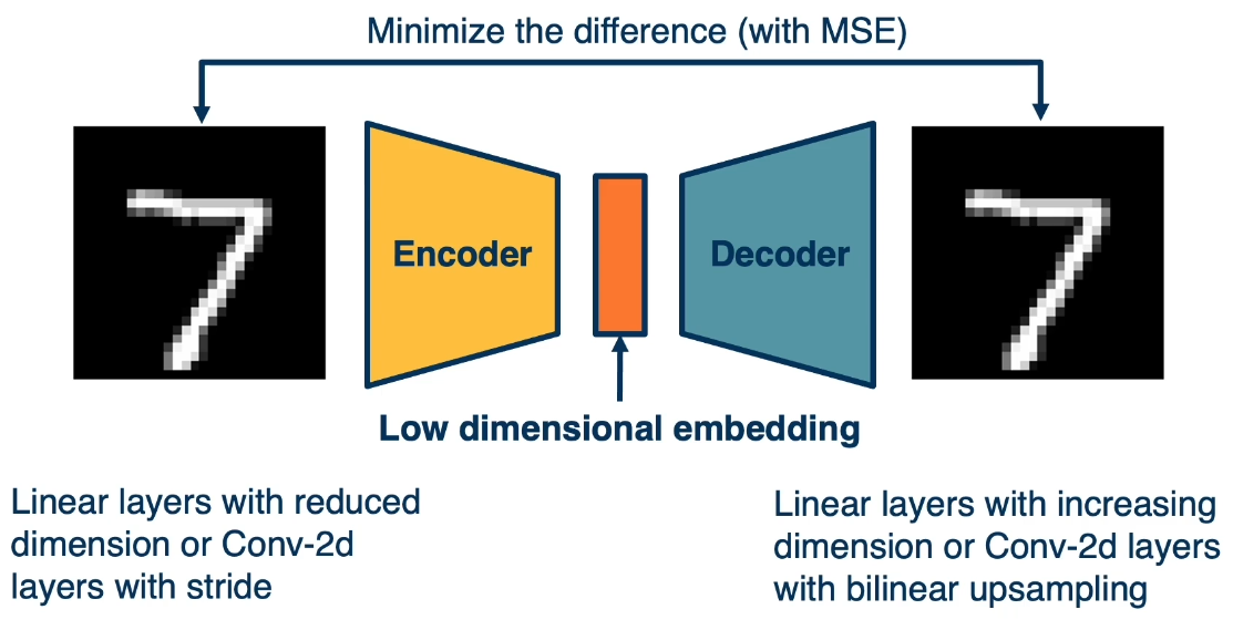
You can then train this using a loss function between the input image and the output image.

To make this generative we replace the hidden representation instead by a probability representation (i.e. outputting the mean and variance of a distribution over the representation). Then we use samples from a fixed distribution $N(0,1)$ multiplied by the outputted probabilities from an input image to generate an input to the decoder. The decoder then outputs an image we can compare against the original.

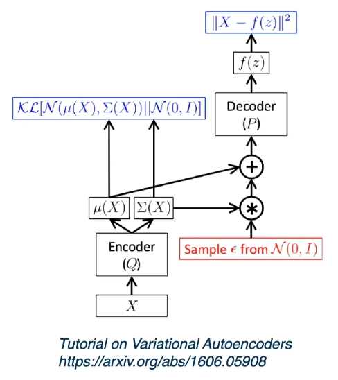
So to summarise we have an encoder $q_{\phi}$ that takes an image and outputs a probability distribution over the hidden representation. Then we have a decoder $p_{\phi}$ that takes a hidden representation and outputs an image - which can be interpreted as a probability distribution over the image’s domain with the output image being the mean and looking at the distribution $N(p_{\phi}(x), 1)$. Now we can do some magic maths to derive a loss function:

$$ \begin{align*} \log p_{\theta}(x^{(i)}) = & \mathbb{E}_{z \sim q_{\phi}(z \vert x^{(i)})} \left [ \log p_{\theta}(x^{(i)}) \right ] & \text{as } p_{\theta} \text{ is a probability distribution}\\ = & \mathbb{E}_z \left [ \log \left ( \frac{p_{\theta}(x^{(i)} \vert z ) p_{\theta} (z)}{p_{\theta}(z \vert x^{(i)})} \right ) \right ] & \text{by Bayes' Rule}\\ = & \mathbb{E}_z \left [ \log \left ( \frac{p_{\theta}(x^{(i)} \vert z ) p_{\theta} (z) q_{\phi}(z \vert x^{(i)})}{p_{\theta}(z \vert x^{(i)}) q_{\phi}(z \vert x^{(i)})} \right ) \right ] & \text{multiplying by a constant}\\ = & \mathbb{E}_z \left [ \log p_{\theta}(x^{(i)} \vert z ) - \log \left ( \frac{q_{\phi}(z \vert x^{(i)})}{p_{\theta}(z) } \right ) + \log \left ( \frac{q_{\phi}(z \vert x^{(i)})}{p_{\theta}(z \vert x^{(i)})} \right ) \right ] & \text{logarithms}\\ = & \mathbb{E}_z \left [ \log p_{\theta}(x^{(i)} \vert z ) \right ] - D_{KL}\left ( q_{\phi}(z \vert x^{(i)}) \vert \vert p_{\theta}(z) \right ) + D_{KL} \left ( q_{\phi}(z \vert x^{(i)}) \vert \vert p_{\theta}(z \vert x^{(i)}) \right ) & \text{definition}\\ \end{align*} $$

The first term here is given by the decoder network i.e. what is the probability of generating the original image given the hidden representation. The second term can also be calculated during back prop by comparing the encoder’s output vs the $z$ prior distribution. The third term is intractable - so instead of getting this exactly we discount it as it is always greater than 0. So this gives us our loss function we use for training, we compare the encoder’s KL divergence against the prior and lastly we compare our decoder’s output against the original image. This can be used in back propagation using a sampling trick where we don’t sample from the encoder directly we instead multiply samples from $N(0,1)$ by the output of the encoder.

Then to generate new images from scratch we can generate random hidden representations and feed them through the decoder. You can nicely show what the hidden layer is encoding by walking that space and putting it through the decoder.

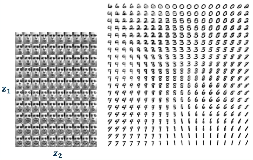
This shows this hidden representation encodes features of your space like the direction a face is pointing or how happy or sad the face is.

Functionally the VAEs outputs are not competitive against GANs but the hidden representations they learn can be useful for downstream tasks such as understanding how a game changes over time.