In this lecture we will look at the application of NLP to machine translation. This can be hard due to multiple factors:

• Sentences are ambiguous like ‘I saw her duck’ or ‘The professor said on Monday we would have an exam’ both could be understood to mean multiple things. So context is important.

• Different languages have different grammatical structure and words that don’t exist in other languages.

• Translation might not be one-to-one instead one to many or many to one.

• There are some ‘markers’ within language that may not exist in others, such as honorific suffixes like ‘-san’ or ‘-chan’ in Japanese, or grammatical gender in French and German.

Translation is traditionally modelled as a conditional language model where we want to calculate $\arg\max_t \mathbb{P}(t \vert s)$ where $t$ is the sentence in the target language and $s$ is the source sentence. Similar to other NLP tasks this can then be broken down as:

$$ \mathbb{P}(t \vert s) = \mathbb{P}(t_1 \vert s) \cdot \mathbb{P}(t_2 \vert t_1, s) \ldots $$

This is worked out in a forward pass. Finding $t_i$ in sequence.

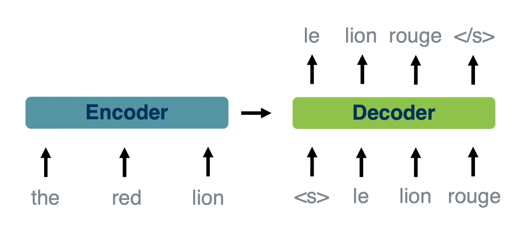
Calculating $\arg\max_t \mathbb{P}(t \vert s)$ is actually intractable so we will use a technique called beam search to check the top 4 to 6 possibilities. The way this works is an encoder-decoder architecture: the encoder reads the source sentence and compresses it into a fixed vector representation, then the decoder autoregressively generates the target sentence token by token conditioned on that representation.

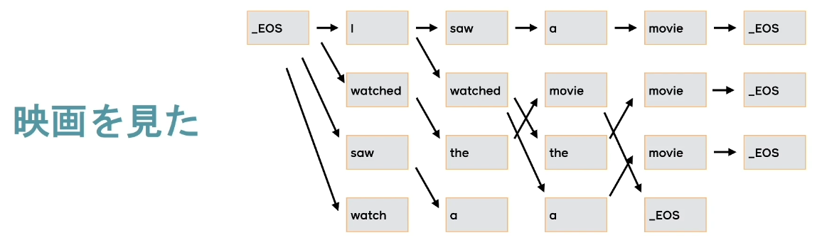
The beam search works by exploring the best $k$ possibilities at each step.

• Each beam element has a different state.

• Total computation scales linearly with the beam width.

• Computation is highly parallelisable between the beams making it efficient.

We use the following kinds of networks for this task:

• RNN: Bi-directional encoder.

• Convolutional: Encoder and decoder based on fixed-width convolutions.

• Transformer: The original encoder-decoder transformer (“Attention is All You Need”) is the dominant architecture for translation. Note that BERT is encoder-only and used for understanding tasks, not generation.

# Inference efficiency

Whilst model developers sink most time into training - ultimately a good model is used for inferring much more than training, so making this optimal is important. This cost comes from:

• Step-by-step computation (auto-regressive inference)

• Output projections: $\Theta(|\text{vocab}| \cdot |\text{output length}| \cdot |\text{beam size}|)$

• Deeper models

This can be mitigated against by:

• Smaller vocabularies,

• More efficient computation, and

• Reduce depth and increase parallelism.

Some methods of vocabulary reduction are choosing a better tokenisation of the language. As well as letting an IBM model (classical statistical MT models from the 1990s that learn word alignment probabilities) subset the output vocabulary for that particular query.

To reduce the depth we can use layer dropout. This randomly drops entire transformer layers (not just attention) during inference, making the model effectively shallower for that pass. Transformers are surprisingly robust to this — the model has learnt redundancy across layers — so the quality degradation is modest while the reduction in serial compute decreases latency and increases parallelism. This does mean the performance is slightly worse though.

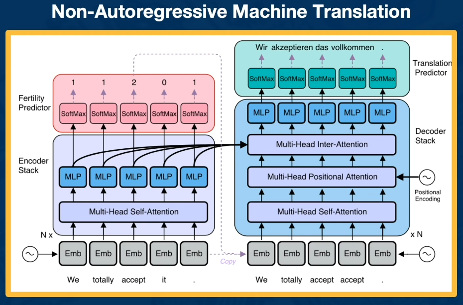
There are newer developments in this area such as non-autoregressive machine translation that instead of predicting one token at a time you predict all tokens at the same time.