In this lecture we will look more at the foundation of attention and relate this to how a transformer works and was built.

# Softmax deep dive

Recall the definition of softmax for a vector $x = \{x_i\}_{i = 1}^N$.

$$ \text{softmax}(x) = (\frac{e^{x_i}}{\sum_{j=1}^N e^{x_j}})_{i = 1}^N $$

This is a probability vector over the entries of $\{x_i\}_{i=1}^N$. There are some interesting things to note about this:

It is sensitive to the relative differences between input values. Multiplying the input by a large constant makes the distribution more peaked, concentrating probability on the largest entry (approaching argmax). Multiplying by a small constant flattens it toward uniform. This is why the scaling factor $\sqrt{d_k}$ matters in attention.
It is order invariant, in the sense that if we switch two inputs their outputs switch but none of the values change.
It is a differentiable approximation of argmax (returning which entry is largest), not max. The differentiable analogue of max is logsumexp: $\log \sum_i e^{x_i}$.

# Attention

The core problem of attention is we have a set of things we want to pay attention to (a set of vectors $u_i$). We have something directing our focus - or a question we want to answer $q$. We now want a way to pick the most relevant $u_i$ to $q$.

If these all existed in a similar vector space then dot product represents un-normalised cosine similarity e.g.

$$ x \cdot y = \cos(\theta_{x,y}) |x| |y| $$

Where $\theta_{x,y}$ is the angle between $x$ and $y$. So $q \cdot u_i$ is a reasonable measure of similarity. Therefore we can use softmax over the dot product to pick one of the $u_i$.

Why not normalise the dot product?

Normalising $q \cdot u_i$ by $|q||u_i|$ would give pure cosine similarity, discarding magnitude. But magnitude carries useful information — a larger $|u_i|$ can signal that a memory is more salient or confident. The softmax denominator already normalises the weights into a probability distribution, so there is no need to also normalise the inputs. More explicitly:

$$ \text{attention}(\{x_i\}, q) = \{\frac{e^{x_i \cdot q}}{\sum_{j=1}^N e^{x_j \cdot q}}\}_{i=1}^N = \text{softmax}(\{x_i \cdot q\}). $$

Softmax as an activation function

When we use softmax at the end of a NN you can see this as an attention calculation where each $u_i$ is a 1-hot embedding of the class $i$. Then $q$ is the last layer of your NN and you want to see which of these classes to pay attention to.

When we have a distribution over the outputs this is called soft attention, though there is hard attention where we pick one. Normally soft attention is used as it is differentiable so it can be used in backpropagation. To go from a distribution to a single output though, we need to then take a weighted sum of the input vectors.

# Soft Attention layers

Now we can use the attention output to define a layer in a neural network. The hidden internal state will be our query vector $q$. Where the $a_i$ are kept fixed. I.e. this layer takes input $x$ and outputs $y$ with some fixed internal values $a_i$:

$$ y = \sum_{i=1}^N \text{attention}(\{a_i\}, x)_i a_i $$

Answering questions

Suppose you are given the following sentences:

1. Brian is a frog.
2. Lily is gray.
3. Brian is yellow.
4. Julius is green.
5. Greg is a frog.

Now you wanted to answer the question ‘What colour is Greg?’ If we use the sentences as our $a_i$ and the question as our first query the following might happen:

Sentence	$q_1$	$q_2$	$q_3$
1	0	0.98	0
2	0.07	0	0
3	0.07	0	1
4	0.06	0	0
5	0.76	0.02	0
In other words, first we make the connection from the question Greg and the word greg in sentence 5.
Next we go from frog in sentence 5 to sentence 1.
Lastly we go from Brian in sentence 1 to sentence 3.
Then there is some idea of a stopping criteria when we have found a colour.
Note here that we will in some way get rid of past inputs so we don’t end up back tracking.

# Transformers

The tag line of transformers is that they are a ‘multi-layer attention model’. This has 3 key advances in how it was designed:

Multi-query hidden-state propagation (“self-attention”)
Multi-head attention
Residual connections, LayerNorm

# Self-attention

With attention layers, we had fixed $u_i$ and we updated a query $q$. However, with self-attention we update the $u_i$ instead of the query.

$$ u^{j+1}_i = \sum_{k=1}^N \text{attention}(\{u^j_k\}, u^j_i)_k u^j_k $$

where $\text{attention}(\{u^j_k\}, u^j_i)_k$ denotes the $k$-th scalar weight in the attention distribution — i.e. how much token $i$ attends to token $k$ at layer $j$.

# Multi-head attention

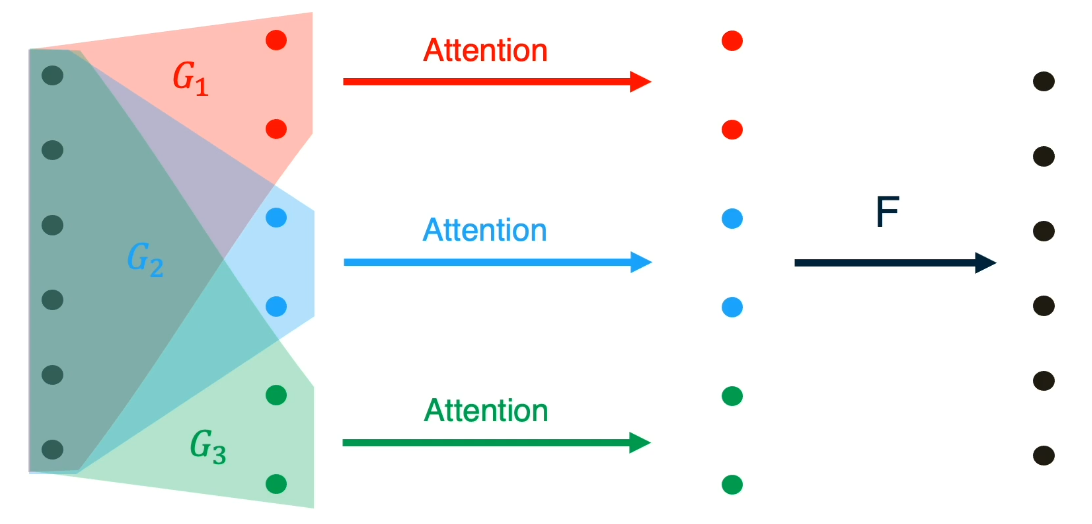
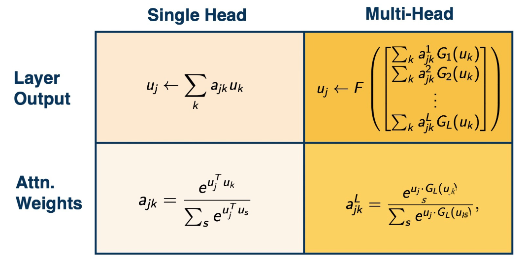
Multi-head attention makes projections from the whole input data to subsets which it runs sub attention layers on. Then at the end it recombines these heads via a fully connected layer to get our output such as below:

Multi-head attention

This has the following equations in different settings.

Multi-head attention equations

# Applications of transformers

Transformers have really revolutionised NLP. Whilst there are applications outside of NLP the most notable examples are all in NLP.

Position encodings depending on the location of a token in the text.
For language models: “causal attention”
Training code outputs a prediction at each token simultaneously (so we can use each token to update the gradient as well to speed up training).

# Week 10 - Neural attention models