# Week 9 - Advanced Indexing Data Structures
Last edited: 2026-07-06
In this lesson we will cover alternatives to hash-tables and B+ tree’s for indexing.
# Trie
For queries that need a pre-fix string matching we use a datastructure built for this. This is called a Trie.
The word “trie” comes from Re’trie’val.
This tree does exactly as you would expect - the internal nodes are prefix characters and the leaves are entries.
In practice we use a Patricia Trie which is the same but instead of storing characters we store sub-words instead.
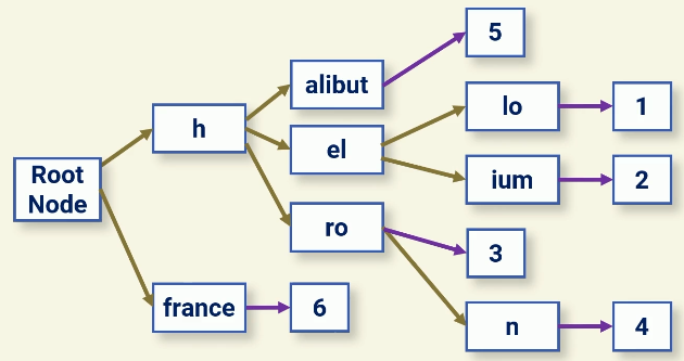
We need the leaf nodes as we may have any entry being a full prefix of another entry for example ‘Hero’ and ‘Heron’ in the above example.
Lets contrast this to a B+ tree. Suppose we have average length of a key as $L$ and the number of the keys as $N$.
| Patricia Trie | B+ Tree | |
|---|---|---|
| Insert | O(L) | O(log N) |
| Search | O(L) | O(log N) |
| Space | O(N*L) | O(N) |
With many keys Patricia Trie becomes faster at inserting and searching but is much larger than a B+ tree.
# Inverted Index
The idea behind a inverted index is the same as the index at the back of a book. It maps from words to their positions within a corpus of text. This normally takes the form of a map from a string to a map from a document number to positions in that document for that word. In C++ we would use the following structure:
class InvertedIndex {
  std::unordered_map<std::string, std::unordered_map<int, std::vector<int>>> index;
  std::vector<std::string> documents;

public:

  void addDocument(int docId, const std::string& content) {
    // Add the document to the collection
    documents.push_back(content);

    // Index the words in the document
    std::vector<std::string> words = split(toLower(contnet));
    for (size_t index = 0; i < words.size(); index++) {
      index[words[index]][docID].push_back(index);
    }
  }

  std::unordered_set<int> getDocuments( const std::string &word) {
    std::string lowerWord = toLower(word);
    std::unordered_set<int> docs;

    // Not found
    if (index.find(lowerWord) == index.end()) {
      return docs;
    }

    // Add all documents that contain the word
    for (const auto &entry : index[lowerWord]) {
      docIDs.insert(entry.first);
    }
    return docs;
  }

  std::unordered_set<int> proximitySearch(const std::string &word1, const std::string &word2, int k) {
    // Finds documents where word1 and word2 appear within k distance of eachother.
  }
};
Inverted indexes are efficient, good for proximity or boolean queries and can scale well. This makes them idea for large document searches such as web search.
# R-tree
A limitation of B+-tree’s is multi-dimensional queries over two numeric indices. The only way B+-trees can handle this is to linearise them i.e. make one numeric value more important than the other. This doesn’t help if we want to answer questions like find all the restaurants in a particular area given by latitude and longitude.
So an R-tree builds on the ideas of a B+-tree but instead of using values as keys it instead uses ‘bounding boxes’
So an R-tree builds on the ideas of a B+-tree but instead of using of storing single values it stores ‘points’ tuples of values. The inner nodes then use bounding boxes that contain the bounding boxes/points of the nodes below it.
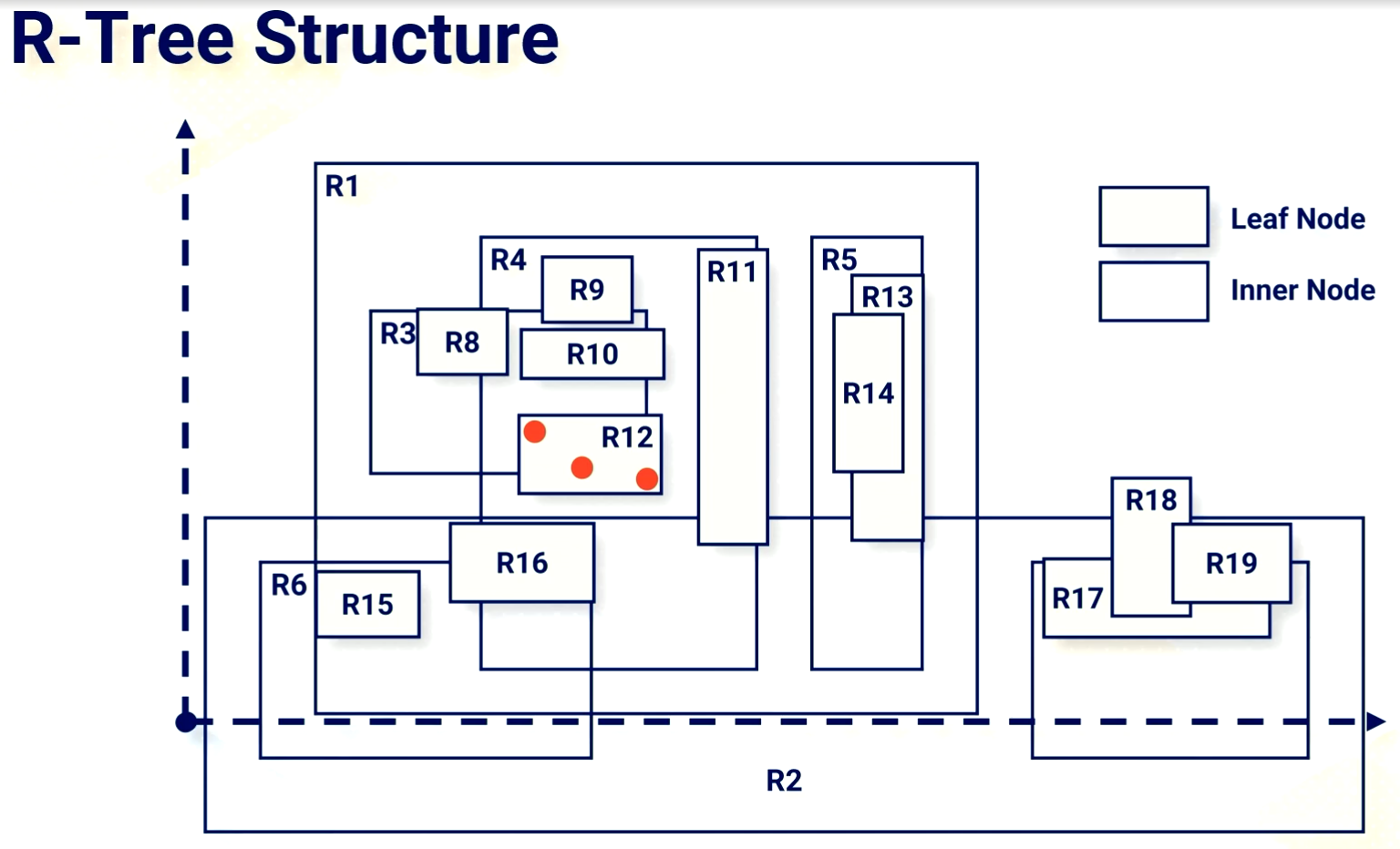
Bounding boxes are defined by 2 extremal points (min and max).
There are 3 types of nodes:
Leaf nodes: These contain a set of points we are storing.
Inner nodes: These point to either Leaf or inner nodes and it maintains a bound box for each child containing all points/bounding boxes in them.
Root node: This has no parent and can have any number of children. Other than that it is the same as an inner node.
Like a B+-tree we ensure a balanced tree. Moreover, we ensure Leaf and Inner nodes have a bounded number of values. When inserting new points we find the leaf node that requires the least enlargement to insert the node into.
Splitting is a little more complicated than a B+-tree. We first pick two points/bounding boxes that are the furthest away. Then we divide the rest of the points by which bounding box would increase the least by adding them. This supports two fast operations:
Range queries: Given a bounding box, you can find all points inside it.
k-Nearest neighbour queries: Given a point, you can find the k-nearest neighbour.
These are both implemented using a depth first search through the tree.
# Learned index
B+ trees practically have a couple of drawbacks:
Fixed structure: The structure leads to multi-level lookup leading to log(n) loopups.
Memory overhead: Each node holds pointers, using a significant memory for large datasets.
Rigid partitions: They do not adapt to predictable key patterns, which can cause unnecessary disk I/O and slower access.
The idea behind a learned index is to use a model to map keys to values (or positions of those values in an array). This can either be a simple regression model or a more complicated neural network. We can still use tree structure to partition key/value pairs to make lookups more accurate and faster.
For the regression model we take the keys and map a line of best fit against the keys/values. Note this might not always be 100% accurate so we my need to search nearby positions in the array to find the precise entry. With this method experimentally we see good performance on both point and range queries.
If the relationships within the nods are not linear simple regression can not perform well. Therefore we night want to use a 1 hidden layer neural network. Here we normalise input and use gradient decent to train each index. This uses MSE as a loss function. The downside to this is the need to train the model and the additional memory it takes to store weights and biases.