Relational databases have uses all across industry. First we motivate why they are useful by comparing it to a flat file database.

# Flat file database

A flat file database keeps all data in flat files - there can be multiple of these each representing individual tables. Then custom code can be written to access or query the data in these files. There are multiple issues with this approach.

# Data redundancy

Without the use of keys within the data, we might need to use data values to link tables together. This not only duplicates the data we are keying but makes it harder to update values across tables.

# Slow operations

Saving the data down to disk means operations such as deleting a row could involve rewriting the entire file. This means a fairly minor operation requires the entire file to be rewritten and saved to disk, which could be very slow.

(There are hardware/software speedups that could speed this up.)

# Slow queries

In CSV format, to do operations such as finding rows with a given value in a column we need to scan the entire file. Again if this file is large this could be very slow. This only gets slower as you want to do more complex operations that use multiple tables.

# Concurrent updates: incorrect data

Concurrent writes to the same file could happen without knowledge of one another - this could lead to incorrect data state. For example, consider two concurrent operations both reading a user’s record: one updates their name, the other updates their location. Without any coordination, one write may overwrite the other, resulting in a lost update — e.g. the name change is silently discarded.

# Handling disk failures

Without a transactional write to disk if a failure occurs it can leave the files in an inconsistent state upon restart. This will mean the data is unrecoverable without manual intervention - which can be hard in large databases.

# Memory management

To speed up operations it will be handy to hold an in memory version of the database. However, this means coordinating writes to disk as the in-memory database changes so we don’t lose changes upon system shutdown.

# Usability

With the use of a flat file, it means writing custom code for each query. This means that the storage layer and the query layer are coupled and makes the data inaccessible to people without a programming background.

# Relational databases

A relational database was introduced by Ted Codd in 1970 who was working as a scientist at IBM. This uses the table abstraction which stores data in a tabular format with pre-specified columns in rows.

Codd’s central motivation was data independence — protecting application programs from being broken by changes to how data is physically stored or organised. He identified three specific data dependencies that existing (tree/network) systems incorrectly coupled programs to:

• Ordering dependence: programs assume data is stored in a particular physical order — if that order changes, programs break.
• Indexing dependence: programs rely on specific indices existing; adding or removing an index breaks them.
• Access path dependence: programs must follow specific named paths through a tree or network structure to traverse data. Codd identifies a concrete failure called the connection trap: following all paths from a given node in a network model gives incorrect results unless the target relation happens to be the natural composition of the others — something that cannot be guaranteed in general.

The relational model eliminates all three by separating the logical design of data (the tables and columns the data owner defines) from the physical design (how data is stored and indexed on disk). The logical layer is expressed in SQL, which does not require a general programming background (though it does require familiarity with query syntax and domain knowledge). This means the database owner can change the physical design — adding indices, reorganising storage — without the data owner needing to know about it.

Another key concept in relational databases is primary/foreign key relations. Each table is provided with a primary key that is used to de-duplicate and link data onto other tables. Tables can contain foreign keys to other tables - the primary key - that links the tables together and ensures there are no empty references.

Together, the logical/physical separation and the primary/foreign key model give relational databases a number of concrete benefits over flat files.

# No data redundancy

Using the primary/foreign key means we no longer need to duplicate fields as references. This makes changes to fields easier to propagate through other tables as well.

# Fast operations

The physical storage can be optimised to speed up common operations. For example, deleting rows can be quick and finding related entries on other tables can cost less using the primary/foreign key relation.

# Fast queries

We can optimise the physical storage - mainly through choosing good indices - to speed up common queries. This can be done in the backend without affecting users’ SQL code.

# Concurrent updates

In a relational database we make changes in transactions which are atomic. Atomicity guarantees that a transaction either commits fully or not at all — no partial changes are visible to other operations. Concurrent transactions are isolated from one another through concurrency control mechanisms (e.g. locking or MVCC), preventing conflicting writes.

# Handling failures

Due to the transactions, we can handle failures such as disk issues. Transactions are saved in totality - so they are either successfully applied or the previous state is known and can be rolled back to.

# Memory management

Relational databases use a Write-Ahead Log (WAL) — changes are recorded to the log before being applied to the data pages on disk. This means that in the event of a crash, committed transactions recorded in the WAL can be replayed to recover the database to a consistent state. Uncommitted transactions at the time of failure are simply discarded.

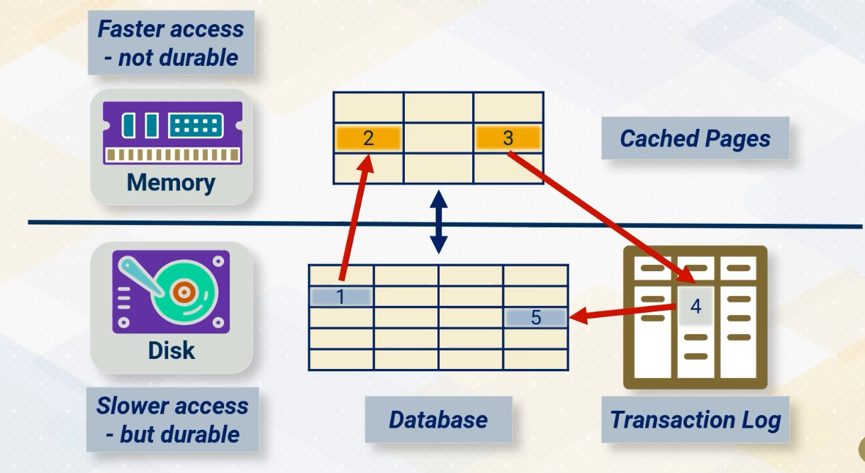
The diagram above shows a row being read into memory, changes are made, these are saved to the transaction log before being applied to the underlying data.

# Usability

Using SQL to access the data reduces the need to write custom code for each query. This allows for the separation between the logical and physical storage of the data.

# Normal form

Codd introduces normalisation to handle relations that contain nonsimple domains — columns whose values are themselves relations (nested or repeating groups) rather than atomic values.

A relation whose domains are all simple (atomic, non-decomposable values) can be represented as a flat two-dimensional array. When a relation has nonsimple domains, this flat representation breaks down and a more complex storage structure is needed. Eliminating nonsimple domains is therefore desirable both for storage and for enabling a universal data sublanguage.

The normalisation procedure works as follows:

1. Start with the top-level relation and take its primary key.
2. Expand each immediately subordinate (nested) relation by inserting this primary key into it.
3. Remove the nonsimple domains from the parent relation.
4. Repeat down the tree until all relations are flat.

employee (man#, name, birthdate, jobhistory, children)
jobhistory (jobdate, title, salaryhistory)
salaryhistory (salarydate, salary)
children (childname, birthyear)

employee' (man#, name, birthdate)
jobhistory' (man#, jobdate, title)
salaryhistory' (man#, jobdate, salarydate, salary)
children' (man#, childname, birthyear)

# Relational operations

Operators function over tables (or sets of relations/tuples). There are standardised operations which we will use in this course, described below in terms of generic relational algebra rather than any specific SQL dialect.

• SELECT ($\pi$): Selects specific columns from a table, removing duplicate rows from the result so the output is a valid relation. Formally $\pi_L(R)$ where $L$ is the list of column indices to keep.

• WHERE ($\sigma$): Filters the rows of a table based on some specific conditions.

• GROUP BY ($\gamma$): Groups the rows of a table based on some specific column values.

• AGG (aggregation) ($\gamma_{agg}$): Aggregates values defined by a GROUP BY clause - common operations include SUM, COUNT, MIN, MAX, and AVG.

• JOIN ($\bowtie$): Links two tables together based on a common key. Formally the natural join $R * S = \{(a, b, c) : R(a, b) \wedge S(b, c)\}$ — combines on a shared domain. Two relations are joinable if such a combining relation exists.

• COMPOSITION ($R \cdot S$): A derived operation — join two relations then project away the shared joining column: $R \cdot S = \pi_{1s}(R * S)$.

• RESTRICTION ($R_{[L|M]}S$): Produces the maximal subset $R'$ of $R$ such that specified columns of $R'$ match the corresponding columns of $S$ — a generalisation of filtering by matching against another relation.

# Relational algebra

Relational algebra allows us to combine the above operations in a way to create more complex queries. This is the theoretical underpinning of operations on relational databases.

*SORT* ($\tau$) TotalLikes DESC
  ($\pi$ PostID, TotalLikes, UsersWhoLiked
    ($\gamma$ COUNT(*) -> TotalLikes,
      GROUP_CONCAT(..) -> UsersWhoLiked
    ($\sigma$ ReactionType = 'like'
      (Interactions) $\bowtie$ Users)
    )
  )

# SQL

SQL is a language that implements this relational algebra. Whilst SQL is referred to as a language it has many ‘dialects’ depending on the application that is implementing it — the core syntax is the same but dialects can add additional syntax or make different choices for what is considered a table identifier or string.

SELECT Interactions.PostID, COUNT(*) AS TotalLikes,
  GROUP_CONCAT(DISTINCT Users.UserID || '-' || Users.Username)
FROM Interactions
JOIN Users ON Interactions.UserID = Users.UserID
WHERE Interactions.ReactionType = 'like'
GROUP BY Interactions.PostID
ORDER BY TotalLikes DESC
LIMIT 1;

PostID, TotalLikes, UsersWhoLiked
1002, 3, 3-alex;4-bella;5-charlie

# Transactions

Above we have discussed transactions but here we go into detail about what their general properties are. At a high level a transaction is a way to safely apply multiple changes to the database as a single unit. This is important when the database must not be left in an invalid intermediate state — for example in banking applications or medical records. To achieve this we say transactions are ACID compliant, we go through each property in more detail below.

# Atomicity

A transaction is atomic if either all the changes happen or none of them do. Exactly the same idea as an atomic operation at the operating system level.

# Consistency

Consistency guarantees that a transaction can only bring the database from one valid state to another valid state — all integrity constraints, foreign key relations, and business rules must hold after every transaction. If a transaction would violate any constraint it is rejected and rolled back, leaving the database unchanged. For example, a bank transfer that would leave an account with a negative balance (violating a non-negative balance constraint) would be rejected in its entirety. This differs from atomicity: atomicity is about whether changes happen at all; consistency is about whether the resulting state is valid.

# Isolation

Isolation guarantees that concurrently executing transactions do not interfere with one another — each transaction sees the database as if it were running alone. For example, suppose two transactions run concurrently: T1 increments a balance by 100 and T2 increments it by 200, both reading an initial balance of 0. Without isolation, both transactions may read the same starting value of 0 and each write their own result independently, leaving the final balance at either 100 or 200 rather than the correct 300. With isolation, the transactions are effectively serialised so that one reads the result of the other, guaranteeing the balance ends at 300.

# Durability

Durability guarantees that once a transaction is successfully committed, that change is permanently stored — it will survive crashes, power failures, or restarts. For example, if a bank commits a transaction that reduces a user’s balance by $500, durability ensures that even if the system crashes immediately afterwards that deduction is not lost when the database recovers.

This is implemented using the WAL (Write-Ahead Log) — a log of all changes that is written to durable storage before the transaction is finalised. On recovery after a crash, the database replays the WAL to restore all committed transactions. Note that a crash before commit simply means the transaction is discarded — the WAL only guarantees committed changes are not lost.